Summarizing Static and Dynamic Big Graphs
Summarizing Static and Dynamic Big Graphs. Arijit Khan Nanyang Technological University, Singapore. Sourav S. Bhowmick Nanyang Technological University, Singapore. Francesco Bonchi ISI Foundation, Italy. Big-Graphs. Google: > 1 trillion indexed pages.

Summarizing Static and Dynamic Big Graphs
E N D
Presentation Transcript
Summarizing Static and Dynamic Big Graphs Arijit Khan Nanyang Technological University, Singapore Sourav S. Bhowmick Nanyang Technological University, Singapore Francesco Bonchi • ISI Foundation, Italy
Big-Graphs Google: > 1 trillion indexed pages Facebook: > 800 million active users Web Graph Social Network 31 billion RDF triples in 2011 31 billion RDF triples in 2011 100M Ratings, 480K Users, 17K Movies De Bruijn: 4k nodes (k = 20, … , 40) Information Network Biological Network Graphs in Machine Learning 1/140
Big-Graph Scales 100M(108) Social Scale 100B (1011) Web Scale 1T (1012) Brain Scale, 100T (1014) US Road Internet Knowledge Graph BTC Semantic Web Web graph (Google) Human Connectome, The Human Connectome Project, NIH 2/140
Why Graph Summarization • Large-scale graph data • - Summarization is critical • Complex graph data • - Interactive and exploratory analysis • - e.g., visualization, pattern mining, anomaly detection 4/140
Why Graph Summarization 1. Memory is getting cheaper 2. Distributed clusters, multi-cores • Large-scale graph data • - Summarization is critical • Fast/ online query processing • Fewer I/O operations • Less data transfer over network • Complex graph data • - Interactive and exploratory analysis • - e.g., visualization, pattern mining, anomaly detection 5/140
Why Graph Summarization • Interactive and exploratory analysis • Approximate query processing • Visualization and visual query interface • Distributed graph processing systems • Processing in modern hardware 6/140
Roadmap • Introduction • Summarizing Static Graphs • Summarizing Dynamic Graphs • Summarizing Heterogeneous Graphs • Summarizing Graph Streams • Domain-dependent Graph Summarization • Future Work and Conclusion 7/140
Categories of Graph Summarization Lossless vs. Lossy Graph Summarization Overlapping vs. Non-overlapping Categories of graphs Summarization techniques Evaluation Metrics 8/140
Categories of Graph Summarization Static graphs Dynamic graphs Stream graphs Lossless vs. Lossy Graph Summarization Overlapping vs. Non-overlapping Homogeneous graphs Heterogeneous graphs Categories of graphs Statistical methods Aggregation-based Attribute-based Compression Application-oriented Summarization techniques Evaluation Metrics 9/140
Categories of Graph Summarization Static graphs Dynamic graphs Stream graphs Lossless vs. Lossy Graph Summarization Overlapping vs. Non-overlapping Homogeneous graphs Heterogeneous graphs Categories of graphs Statistical methods Aggregation-based Attribute-based Compression Application-oriented Summarization techniques Summarization for graph workloads Domain-specific summarization Evaluation Metrics
Categories of Graph Summarization Static graphs Dynamic graphs Stream graphs Lossless vs. Lossy Graph Summarization Overlapping vs. Non-overlapping Homogeneous graphs Heterogeneous graphs Categories of graphs Statistical methods Aggregation-based Attribute-based Compression Application-oriented Summarization techniques Space Efficiency Accuracy Interestingness Summarization for graph workloads Domain-specific summarization Evaluation Metrics
Graph Summary: Varieties of Graphs • Homogeneous graphs • - summarize only topology information (nodes + edges) • Heterogeneous graphs • - nodes and edges have different types and attributes • - summarization happens at both structural and semantic levels 12/140
Graph Summary: Varieties of Graphs • Homogeneous graphs • - summarize only topology information (nodes + edges) • Heterogeneous graphs • - nodes and edges have different types and attributes • - summarization happens at both structural and semantic levels • Static graphs Types of Temporal/ Evolving Networks • Dynamic graphs • Stream graphs 13/140
Graph Summary: Varieties of Graphs • Homogeneous graphs • - summarize only topology information (nodes + edges) • Heterogeneous graphs • - nodes and edges have different types and attributes • - summarization happens at both structural and semantic levels • Snapshots of graph over time • Snapshots are given apriori • can perform many passes over snapshots to build summary • Static graphs Types of Temporal/ Evolving Networks • Dynamic graphs • Edge-streams arriving in real-time • One pass over the stream to incrementally build/ update the summary • Stream graphs
Graph Summarization Techniques • Statistical methods • - degree distribution, hop-plot, clustering coefficient • Aggregation-based • - grouping of nodes and edges into super-nodes/ super-edges • Attribute-based • - summary considering both topology and attributes (heterogeneous graphs) • Compression • - reducing storage space by smartly encoding nodes and edges • Application-oriented • - summarization for efficient graph querying (e.g., shortest path, graph pattern matching) • - domain-specific (e.g., bioinformatics, visual querying) 15/140
Challenges in Graph Summarization • Varieties of graph data • - static vs. dynamic vs. stream • - homogeneous vs. heterogeneous • - numerical vs. categorical attributes • No unique graph summarization technique! • Different objectives • - OLAP vs. compression • - Lossy vs. lossless summary • - Accuracy vs. efficiency vs. space • Different applications/ workloads/ systems • - shortest path vs. graph pattern matching • - main-memory vs. distributed 16/140
This tutorial is not about … • Other related graph analytics, e.g., • - Clustering • - Sampling • - Sparsification • - Community detection • - Graph embedding • - Partitioning • - Dense subgraph mining • - Frequent subgraph mining • …… • Graph compression • - Webgraph compression [Boldi & Vigna, WWW 2004; Raghavan & Molina, ICDE 2003] • - Shingle ordering [Chierichetti et al., KDD 2009] • - Layered label propagation [Boldi et al., WWW 2011] • - k2 Tree [Brisaboa et al., SPIRE 2009] • Summarization for graph workloads • - Reachability and subgraph pattern matching [Fan et al., SIGMOD 2012] • - Keyword search [Wu et al., VLDB 2013] • - Neighborhood query [Maserrat et al., KDD 2010] • - Entity resolution/ Deduplication [Zhu et al., ISWC 2016] • …… 17/140
This tutorial is not about … • Other related graph analytics, e.g., • - Clustering • - Sampling • - Sparsification • - Community detection • - Graph embedding • - Partitioning • - Dense subgraph mining • - Frequent subgraph mining • …… • Distributed graph summarization • - Liu et al., CIKM 2014 • - Junghanns et al., BTW 2017 • …… • Statistical methods • - Degree distribution, hop-plot, clustering coefficient • - Graph generative models • [Chakrabartiet al., ACM Comp. Survey 2006] • …… • Graph compression • - Webgraph compression [Boldi & Vigna, WWW 2004; Raghavan & Molina, ICDE 2003] • - Shingle ordering [Chierichetti et al., KDD 2009] • - Layered label propagation [Boldi et al., WWW 2011] • - k2 Tree [Brisaboa et al., SPIRE 2009] • We shall not discuss them • Summarization for graph workloads • - Reachability and subgraph pattern matching [Fan et al., SIGMOD 2012] • - Keyword search [Wu et al., VLDB 2013] • - Neighborhood query [Maserrat et al., KDD 2010] • …… 18/140
Other Related Tutorials/ Surveys • [Tutorial] S.-D. Lin, M.-Y. Ych, and C.-T. Li, Sampling and Summarizing for Social Networks, in SDM 2013 • [Tutorial] D. Koutra, Summarizing Large-Scale Graph Data, in SDM 2017 • [Survey] Y. Liu, A. Dighe, T. Safavi, and D. Koutra, A Graph Summarization: A Survey, in ArXiv 19/140
Other Related Tutorials/ Surveys • Our New Materials: • Summarizing dynamic and stream graphs • Domain-dependent graph summaries • [Tutorial] S.-D. Lin, M.-Y. Ych, and C.-T. Li, Sampling and Summarizing for Social Networks, in SDM 2013 • [Tutorial] D. Koutra, Summarizing Large-Scale Graph Data, in SDM 2017 • [Survey] Y. Liu, A. Dighe, T. Safavi, and D. Koutra, A Graph Summarization: A Survey, in ArXiv 20/140
Other Related Tutorials/ Surveys • Our New Materials: • Summarizing dynamic and stream graphs • Domain-dependent graph summaries • [Tutorial] S.-D. Lin, M.-Y. Ych, and C.-T. Li, Sampling and Summarizing for Social Networks, in SDM 2013 • [Tutorial] D. Koutra, Summarizing Large-Scale Graph Data, in SDM 2017 Specific sub-areas under graph summarization • [Survey] Y. Liu, A. Dighe, T. Safavi, and D. Koutra, A Graph Summarization: A Survey, in ArXiv • Y. Liu, N. Shah, and D. Koutra, An Empirical Comparison of the Summarization Power of Graph Clustering Methods, in ArXiv, 2015 • A. McGregor, Graph Stream Algorithms: A Survey, in SIGMOD Rec., 2014 • C. Chen, C. X. Lin, M. Fredrikson, M. Christodorescu, X. Yan, and J. Han, Mining Large Information Networks by Graph Summarization, in Link Mining: Models, Algorithms, and Applications, 2010 • Y. Tian and J. M. Patel, Interactive Graph Summarization. In Link Mining: Models, Algorithms, and Applications, 2010
Roadmap • Introduction • Summarizing Static Graphs • Summarizing Dynamic Graphs • Summarizing Heterogeneous Graphs • Summarizing Graph Streams • Domain-dependent Graph Summarization • Future Work and Conclusion 22/140
Summarizing Static Graphs SIGMOD 08 SDM 10 • Summary made of supernodes (set of nodes) and superedges • Follow the MDL principle • Lossy • Densities • Number of supernodes predefined • Answer queries directly on the summary (expected-value semantics) • Both lossless or lossy (with bounded error) • Edge corrections 23/140
i h j i h j Cost = 14 edges d e f g • Compression possible (S) • Many nodes with similar neighborhoods • Communities in social networks; link-copying in webpages • Collapse such nodes into supernodes (clusters) and the edges into superedges • Bipartite subgraph to two supernodes and a superedge • Clique to supernode with a “self-edge” • Need to correct mistakes (C) • Most superedges are not complete • Nodes don’t have exact same neighbors: friends in social networks • Remember edge-corrections • Edges not present in superedges (-ve corrections) • Extra edges not counted in superedges (+ve corrections) • Minimize overall storage cost = S+C a b c Summary X = {d,e,f,g} Y = {a,b,c} Corrections Cost = 5(1 superedge + 4 corrections) 24/140
i h j Representation Structure R=(S,C) Summary X = {d,e,f,g} • Summary S(VS, ES) • Each supernode v represents a set of nodes Av • Each superedge (u,v) represents all pair of edges πuv = Au x Av • Corrections C: {(a,b); a and b are nodes of G} • Supernodes are key, superedges/corrections easy • Auv actual edges of G between Au and Av • Cost with (u,v) = 1 + |πuv – Auv| • Cost without (u,v) = |Auv| • Choose the minimum, decides whether edge (u,v) is in S • Reconstructing the graph from R • For all superedges (u,v) in S, insert all pair of edges πuv • For all +ve corrections +(a,b), insert edge (a,b) • For all -ve corrections -(a,b), delete edge (a,b) Y = {a,b,c} C = {+(a,h), +(c,i), +(c,j), -(a,d)} d e f g h i j a b c d e f g h i j a b c 25/140
Greedy • Cost of merging supernodes u and v into single supernode w • Recall: cost of a superedge (u,x): c(u,x) = min{|πvx – Avx|+1, |Avx|} • cu = sum of costs of all its edges = Σx c(u,x) • s(u,v) = (cu + cv – cw)/(cu + cv) • Main idea: recursive bottom-up merging of supernodes • If s(u,v) > 0, merging u and v reduces the cost of reduction • Normalize the cost: remove bias towards high degree nodes • Making supernodes is the key: superedges and corrections can be computed later u v w cu = 5; cv =4 cw = 6 (3 edges, 3 corrections) s(u,v) = 3/9 26/140
Greedy Cost reduction: 11 to 6 bc a d • Recall: s(u,v) = (cu + cv – cw)/(cu + cv) • GREEDY algorithm • Start with S=G • At every step, pick the pair with max s(.) value, merge them • If no pair has positive s(.) value, stop ef gh C = {+(h,d),+(a,e)} b bc bc c a a a d d d e e e h h f gh f f g g C = {+(h,d)} s(b,c)=.5[ cb = 2; cc=2; cbc=2 ] s(g,h)=3/7[ cg = 3; ch=4; cgh=4 ] s(e,f)=1/3[ ce = 2; cf=1; cef=2 ] 27/140
Randomized • GREEDY is slow • Need to find the pair with (globally) max s(.) value • Need to process all pair of nodes at a distance of 2-hops • Every merge changes costs of all pairs containing Nw • Main idea: light weight randomized procedure • Instead of choosing the globally best pair, • Choose (randomly) a node u • Merge the best pair containing u 28/140
Randomized b c a d e • Randomized algorithm • Unfinished set U=VG • At every step, randomly pick a node u from U • Find the node v with max s(u,v) value • If s(u,v) > 0, then merge u and v into w, put w in U • Else remove u from U • Repeat till U is not empty h f g Picked e; s(e,f)=3/5[ ce = 3; cf=2; cef=3 ] b c a d h ef g C = {+(a,e)} 29/140
Approximate Representation Rє X = {d,e,f,g} Y = {a,b} • Approximate representation • Recreating the input graph exactly is not always necessary • Reasonable approximation enough: to compute communities, anomalous traffic patterns, etc. • Use approximation leeway to get further cost reduction • Generic Neighbor Query • Given node v, find its neighbors Nv in G • Apx-nbr set N’vestimates Nv with є-accuracy • Bounded error: error(v) = |N’v\Nv| + |Nv\N’v| < є |Nv| • Number of neighbors added or deleted is at most є-fraction of the true neighbors • Intuition for computing Rє • If correction (a,d) is deleted, it adds error for both a and d • From exact representation R for G, remove (maximum) corrections s.t.є-error guarantees still hold C = {-(a,d), -(a,f)} d e f g a b For є=.5, we can remove one correction of a d e f g a b 30/140
Computing approx representation S • Reducing size of corrections • Correction graph H: For every (+ve or –ve) correction (a,b) in C, add edge (a,b) to H • Removing (a,b) reduces size of C, but adds error of 1 to a and b • Recall bounded error: error(v) = |N’v\Nv| + |Nv\N’v| < є |Nv| • Implies in H, we can remove up to bv = є |Nv| edges incident on v • Maximum cost reduction: remove subset M of EH of max size s. t. M has at most bv edges incident on v • Same as the b-matching problem • Find the matching M EGs.t. at most bv edges incident on v are in M • For all bv = 1, traditional matching problem • Solvable in time O(mn2) [Gabow-STOC-83] (for graph with n nodes and m edges) C Cє 31/140
Computing approx representation S • Reducing size of summary • Removing superedge (a,b) implies bulk removal of all pair edges πuv • But, each node in Au and Av has different b value • Does not map to a clean matching-type problem • A greedy approach • Pick superedges by increasing |πuv| value • Delete (u,v) if that doesn’t violate є-bound for nodes in AuUAv • If there is correction (a,b) for πuv in C, we cannot remove (u,v); since removing (u,v) violates error bound for a or b Sє Cє 32/140
APXMDL S C • Compute the R(S,C) for G • Find Cє • Compute H, with VH=C • Find maximum b-matching M for H; Cє=C-M • Find Sє • Pick superedges (u,v) in S having no correction in Cєin increasing |πuv| value • Remove (u,v) if that doesn’t violate є-bound for any node in Au U Av • Axp-representation Rє=(Cє, Sє) Sє Cє 33/140
Reduces the cost down to 40% Cost of GREEDY 20% lower than RANDOMIZED RANDOMIZED is 60% faster than GREEDY 34/140
Summary Node partition Original graph Adjacency matrix of the original graph Expected adjacency matrix resulting from the summary 35/140
Query answering • Queries to the original graph can be approximated directly on the summary. • The expected adjacency matrix can be seen as a probabilistic (uncertain) graph. • Expected value sematics • Example: • Expected degree of node #2: • 2/3 + 2/3 + 1/3 + 1/3 = 2 • Other measures: • Expected eigenvector centrality • Expected number of triangles* • * [Riondato et al., ICDM’14, DMKD] 36/140
Minimize the reconstruction error • A summary is good when the expected adjacency matrix is close to the original adjacency matrix • Define reconstruction error as the difference between the two matrices. • Problem*:given an integer k find a k-partiton of the nodes s.t. the corresponding summary minimizes reconstruction error. * LeFevre & Terzi also define a MDL-based variant with no k parameter. 37/140
Greedy algorithm • Greedy agglomerative hierarchical clustering: 1) Put each vertex in a separate supernode; 2) Until the number of supernodes is k: • Merge the two supernodeswhose merging minimizes the reconstruction error; 3) Output the resulting k supernodes; • Main limitations: • no quality guarantees • very slow 38/140
Riondato et al. ICDM’14 DMKD • Overcome GraSS limitations: fast algorithm with constant-factor approximation guarantee • Generalize reconstruction error to • Consider cut-norm error • Among the contributions: a practical use of extreme graph theory, with the cut-norm and the algorithmic version of Szemerédi’s Regularity Lemma. 39/140
Roadmap • Introduction • Summarizing Static Graphs • Summarizing Dynamic Graphs • Summarizing Heterogeneous Graphs • Summarizing Graph Streams • Domain-dependent Graph Summarization • Future Work and Conclusion 42/140
IEEE BigData 2016 • Extends the GraSS framework to dynamic graphs • Dynamic graph = a tensor with one dimension increasing in time • Potentially infinite stream of static graphs • Define a sliding tensor window • Summarize the tensor within the tensor window 43/140
Overview and contributions • At each time-stamp : • A new adjacency matrix arrives • The sliding window is updated (one adjacency matrix exits the window) • Summary is created for the current window, by clustering nodes to creatsupernodes (following Riondato et al.) • Output: one summary at every time-stamp • Contributions: • Two online algorithms for summarizing dynamic, large-scale graphs • Distributed, scalable algorithms, implemented in Apache Spark
Algorithms • Baseline: • Standard k-means clustering at each timestamp • N points each with wN values • Observation: (w-1)N2unchanged at every new timestamp • Two-level clustering: • adjacency matrix to micro-clusters • keep statistics in the micro-clusters • run maintenance algorithm • micro-clusters to supernodes
KDD’15 • Use a dictionary of temporal templates: - Static templates - Temporal signatures • Get the shortest lossless description (MDL) - Better compression better summary bip. core near clique chain star near bip. core clique flickering constant oneshot periodic ranged x x x x 46/140
Formal goal … • Given a dynamic graph G temporal templates Φ, • Findthe smallest model M s.t. min L(G,M) = L(M) + L(E) G1 G2 Gn Error E Adjacency A Model M time
Proposed algorithm: TimeCrunch • Step 1: Generate static subgraph instances G1 G2 G3 bc bc bc st st fc fc fc 48/140
Proposed algorithm: TimeCrunch • Step 1: Generate static subgraph instances • Step 2: Stitch static instances together to form temporal instances G3 G1 G2 constantbc bc bc bc st st flickeringst constant fc fc fc fc 49/140