Multivariate Analysis of Variance, Part 1

1. Multivariate Analysis of Variance, Part 1 BMTRY 726

2. >2 Independent Samples What happens if we have more than two independent populations we want to compare?

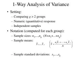
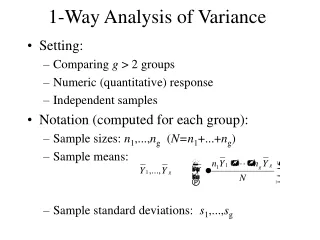
3. Review ANOVA Given a random sample We rewrite ml as the overall mean plus the treatment effect of treatment l Thus we end up testing Using the model Grand mean Treatment effect Error Sample mean Est. treatment effect Residual

4. What we want to answer… is the contribution of the treatment large relative to our residuals? In ANOVA we do this using the sums of squares:

5. What we want to answer… is the contribution of the treatment large relative to our residuals? In ANOVA we do this using the sums of squares:

6. >2 Samples for MVN We can use one-way MANOVA to compare mean vectors for our g populations. Assumptions: (1) Independent random samples from g groups (2) Homogeneity of covariance matrices (3) Normality Summary Statistics:

7. One-way MANOVA Pooled estimate of the common covariance matrix: One-way MANOVA model:

8. One-way MANOVA Compute summary statistics for each sample SAS constraint: Vector of random errors that are ~NID(0,S) Mean vector for the lth population ml = m + tl Vector of obs for jth unit Selected from lth population

9. One-way MANOVA We can write the multivariate version of the sums of squares now… So if we want to test if all treatment effect are equal: Total SS and cross products Between (trt) SS and cross products Within (resid) SS and cross products

10. One-way MANOVA We reject out null hypothesis of Wilk’s lambda is too small. Under certain conditions, the exact distribution of lambda is known: -see table 6.3 on page 303 For other cases and when n is large, we can use the Bartlett modification

11. Distribution of L* • Sampling distribution for MVN data No. of No. of Sampling distribution for MVN data variables groups

12. Example: Infant Right Ventricular Failure An investigator examines the at the effect of giving H2S to rabbits with banded right ventricles on heart tissue “floppiness” and amount of oxidized cystine residues in mitochondria collected from heart tissue. There are three groups of animals (1) Banded and untreated (2) Banded but dosed with H2S (3) Banded and over-express CES to produce H2S There are 3 rabbits in each group.

13. Example

14. Example

15. Example

16. Example

17. Example

18. Example

19. Confidence Intervals If we reject the null hypothesis, we want to determine which treatments are different. In this case, the Bonferroni approach applies We use this to develop an expression for the CI difference between treatment k and l

20. Example Estimate the 95% CIs for each treatment difference

21. Example Estimate the 95% CIs for each treatment difference

22. MANOVA as Linear Model If we think about is as a linear model…

23. Model Features • Each row of the error matrix (or each row of X) -is independent of any other row -has covariance matrix S • Each column of X -corresponds to a different trait -has a model for the mean of the same form -has a corresponding column of parameters in the design matrix

24. MANOVA MLE’s Maximum likelihood estimates of parameters in b: For the PROC GLM version of the one-way MANOVA

25. The jth column of contains parameter estimates for the model fit to the data for the jth trait:

26. Kronecker product:

27. Inference We can make certain inferences about the elements of our parameter matrix Generalized LRT procedure (Wilks, 1932) Make comparison across groups (rows of b) Make comparisons across traits Matrix of zeros

28. Compute the corrected sums of squares and cross-products matrix for the model: • This reduces to: • The diagonal elements of H are model sums of squares whenM = I:

29. Compute a matrix of residual sums of squares and cross-products: When M = I: Diagonal elements of E are sums of the squared residuals Off-diagonal elements are sums of cross-products of residuals

30. Likelihood Ratio Test Reject the null hypothesis if Wilk’s criterion is too small Large sample chi-square approximation, reject H0 if

31. A more accurate approximation given by Rao (C.R. Rao (1951) Bull Int Stat Inst. 33(2), 177-180.) When is true: where

32. Exact distribution of Wilk’s criterion: (1) Independence (2) Homogeneity of covariance matrices (3) Multivariate normality When is true: When either These are the cases in Table 6.3 on page 303 In J & W

33. Other Criteria Wilk’s Lambda: Lawely-Hotelling Trace Pillai Trace Roy’s Maximum Root:

34. Example Recall our example right ventricular failure example…

35. Example Our estimate of b … Say we want to test the hypothesis of equal treatment effects:

36. Example We have to find E and H …

37. Example We have to find E and H …

38. Example We can use E and H to find lambda… Does this match what we calculated using our MANOVA table? NOTE: If pand gmatch conditions in table 6.2, we can compare this to the F distribution. Otherwise we can use the c2 approximation if nis large.