Stochastic Process

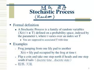
1. Stochastic Process • Formal definition • A Stochastic Process is a family of random variables {X(t) | t  T} defined on a probability space, indexed by the parameter t, where t varies over an index set T • You are supposed to associated T with time • Examples • Frog jumping from one lily pad to another 　 X(t) = lily pad occupied by the frog at time t • Flip a coin and take one step north if heads and one step south if tails（discrete time , discrete state） • 股票, 天氣

2. arrivals Server departures Queue on waiting room Queuing Systems as stochastic processes • Single server model • Arrival process • Queue scheduling discipline • Service time distribution System

3. Some random processes associated with a queuing system Continuous time random processes • X(t) ＝ # of arrivals in （0, t） • N(t) ＝ # of customs(jobs) in system at time t • X(tn) ＝ # of customs(jobs) in system when nth arrival occurs • U(t) ＝ amount of unfinished work in the system at time t Discrete time random process Continuous time random process

4. Markov ??? M/M/1/N • M： Arrival：Poisson Service：Exponential • G：General • D：Deterministic Arrival process # of servers Service time distribution Finite waiting room Memoryless

5. Fig 2.2 Cn-1 Cn Cn+1 Cn+2 • Wn = nth customer’s waiting time(inside the queue) • Xn = nth customer’s service time(inside the server) • System time = waiting time + service time Xn+1 Xn+2 Xn idle Server Cn Cn+1 Cn+2 Wn Wn+1 Wn+2=0 Queue Cn Cn+1 Cn+2

6. Little’s ResultλT=n • Def: • λ：mean long term arrival rate (no assumption about Poisson or anything else -not even i.i.d. interarrival times) • T：mean time a customer spends in the black box • n：mean number of customers in the box Black box arrivals departures

7. Proof customers Err T5 T4 T3 T2 T1 time 0 t Err

8. Let • n(t) = # of cistomers in the system at time t • A(t) = # of arrivals in (0, t) • # of customers in the system= area

9. ‾= n ‾= n t→∞, 只要 steady state, Err(t) won’t grow up ∴ , as t →∞

10. Stochastic Processes • Notation: F(x0;t0) = FX(t0)(x0) = P[X(t0) ≦x0] • Describing stochastic processes • F(x1, x2,…, xn; t1, t2,…, tn) = F(x; t) =P[X(t1) ≦ x1, X(t2) ≦ x2,…, X(tn) ≦ xn] Sample path Distrib of initial state τ τ 0 t1 t2 t

11. Special case • Stationary • F(x;t)=F(x; t + τ), where t + τ = t1 + τ, t2 + τ, …, tn + τ • Independent • F(x; t)=Fx(t1)(x1)Fx(t2)(x2)…Fx(tn)(xn)

13. Markov Processes • Future behavior does not depend on all of past history • Only depends on current state • P[X(t) = x|X(t1) = x1,…, X(tn) = xn] =P[X(t) = x| X(tn) = xn], t1<t2<…<tn<t • Concerned mostly with discrete state Markov Chains • Discrete and continuous time • Time homogeneous Markov processes • P[X(t) ≦ x| X(tn) ≦xn]=P[X(t + τ) ≦ x| X(tn + τ) ≦xn], for all τ

14. Markov Chins --discrete state space • May be continuous time or discrete time p12 2 p24 p23 p14 1 4 p44 p13 p31 p43 3

15. Markov Chain • For discrete parameter • We only consider the sequence of states and not the time spent in each state • For continuous time M.C. • The “holding time” in each state is exponential distributed • Must be if future behavior only depends on current state • Need the memoryless property of the exponential

16. Discrete time M.C. • P = transition probability Matrix • P[i, j] = p[X(t+1) = j | X(t) = i] • Continuous time M.C. • Rate of transmission between states

17. p1 m1 q1 Interconnect p2 m2 q2 qm pn mm How to select state? • Ex: • Model of a shared memory multiprocessors

18. m1 ?? q1 ?? m2 q2 qm ?? mm How to select state? (cont.) • An abstraction

19. < (p1, p2), (　 ) > 1 < ( p1 ), ( p2 ) > 2 < ( p2 ), ( p1 ) > 3 < (p2,p1), ( ) > 4 < ( ), (p1, p2) > 5 < ( ), (p2,p1) > 6 How to select state? (cont.) • Parameter case • 2 processors • 2 memory modules ?????? ??????

20. Discrete Parameter Markov Chains • Discrete state space • Finite or countable infinite • Pjk(m, n) = P[Xn = k | Xm = j], 0 ≦ m ≦ n • For time homogeneous Markov Chains • Pjk(m, n) is only a function of n-m • In particular,Pjk = Pjk(m, m+1)

21. Transition probability matrix • P = P[j, k] (stochastic matrix) • All elements ≧ 0 and row sums = 1 • π(0) = initial state probability vector • πi(0)= ith component of π(0) = prob. system starts in state i

22. 12 12 12 12 0 0 0 12 12 12 j i Xn-1 Xn State-transition diagram • Example: Random walk • N-step Transition Probabilities • Def: n-step transition prob. matrix

24. 1 transient Type of states & types of Markov Chains • Transient states • “no way to go back” • “1” is a transient state • Pji(n) → 0, as n →∞

25. Recurrent states • 相反於 transient • State i is recurrent iff starting from any state j, state i is visited eventually with probability 1. Pji(n) → 1, as n →∞ • Expectation is ∞ • Recurrent-null • Mean time between visits is ∞ • Recurrent-non-null • Mean time between visits is < ∞ • Periodic • di=g.c.d of all n such that Pii(n) ≠ 0 • aperiodic if di = 1

26. Absorbing states • “trap states“ • “4” is an absorbing state, so is “5” p 4 7 5 1-p

27. Irreducible Markov Chain • Any state is reachable from any other state in a finite number of transition, • i.e. vi, j, Pij(n) > 0 for some finite n • For an irreducible Markov chain • All states are aperiodic or all are periodic with the same period • All states are transient or none are • All states are recurrent or none are

28. Let π(0) = vector of initial state probabilities • i.e. πi(0) = prob. start in state i 　　πi(0) = prob. in state i at time = 1

30. Thm. • For any aperiodic chain, the limit • Thm. • For an irreducible, aperiodic M.C., the limit of πexists and is independent of the initial state probability distribution • Thm. • For an irreducible, aperiodic M.C. with all states recurrent non-null, πis the unique stationary state probability vector

31. 1 A B 1 1 C Example • Limit does not exist for a periodic chain: • π(0) = (1, 0, 0) • π(3k) = (1, 0, 0) • π(3k+1) = (0, 1, 0) • π(3k+2) = (0, 0, 1) no limit

32. A B C D A B C D Example • Reducible M.C: • Solution to π= πP is not independent of initial state prob. Vector • π(0) = (1, 0, 0, 0) Or π(0) = (0, 0, 1, 0) B D A C

33. q1 p1 m1 Interconnect q2 p2 m2 q1 (2, 0) (1, 1) (0, 2) (2, 0) q2 q12 (2, 0) (1, 1) 1-q12-q22 q22 (1, 1) q1 (0, 2) (0, 2) Recall: problem before --2 memory modules case and 2 processors • Step 1: select state • (2, 0) (1, 1) (0, 2) • Step 2: transition P => q1 P1p2 m1 q2 m2 q2

34. Step 3: 求π • π= πP • Σ πi = 1 令π=(π1, π2, π3) • (π1, π2, π3) = (π1, π2, π3)

35. Performance measure • Usually expressed as “reward functions” • E.q. memory bandwidth: • i.e.expected # of references completed per cycle = π(2, 0)‧1 + π(0, 2)‧1 + π(1, 1)‧2

36. a0 a1 a2 b0 b1 b2 0 1 2 d1 d2 d3 Discrete Parameter Birth-Death Process • bi = prob. of a birth in state i • di = prob. of a death in state i • ai = prob. of a neither in state I • π= πP • Straight form above eqn

37. Substitute imploes.

38. Messy with all the b.d.a. arbitrary

40. Σ pik = 1 pji πj j pik i πi j πj • 另解 • π= πP（by balance equation）

41. πjPji= • ‘rate’ at which state i is entered from state j • ∴ Σj πjPji= total ‘rate’ into state i • πj = fraction of visits to state i = ‘rate’ at which state i is exited • πi = Σj πjPji（π= πP）

43. a0 a1 a2 ai ai+1 b0 b1 b2 bi bi+1 0 1 2 i i+1 d1 d2 d3 di+1 di+2 • Another way of solving • --sometimes were convenient • πi bi = πi+1 di+1 πi+1 = （ bi∕ di+1）πi

45. Examples • An infinite stack • A finite stack • Two stacks growing toward each other

46. Some properties of Poisson processes • Alternate Def. • N(0) = 0 • Independence of non-overlapping intervals • Time homogeneity • P[1 event in (t, t+h)] = λh + o(h) • P[0 event in (t, t+h)] = 1- λh +o(h) • P[ > 1 event in (t, t+h)] = o(h)

47. t+h 0 t t+h • Maybe • 0 event • 1 event • 2 events (p → 0)

48. Poisson λA What distribution? Still Poisson? λz Poisson • Merging independent Poisson processes

50. ? A λ What distribution? Still Poisson? Poisson Z ? • Splitting a Poisson process