
Reference : (see course web site) Sample PSPICE Report
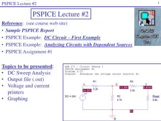
PSPICE Lecture #2. 1. PSPICE Lecture #2. Reference : (see course web site) Sample PSPICE Report PSPICE Example: DC Circuit – First Example PSPICE Example: Analyzing Circuits with Dependent Sources PSPICE Assignment #1. Topics to be presented : DC Sweep Analysis

Reference : (see course web site) Sample PSPICE Report
E N D
Presentation Transcript
PSPICE Lecture #2 1 PSPICE Lecture #2 • Reference: (see course web site) • Sample PSPICE Report • PSPICE Example: DC Circuit – First Example • PSPICE Example: Analyzing Circuits with Dependent Sources • PSPICE Assignment #1 • Topics to be presented: • DC Sweep Analysis • Output file (.out) • Voltage and current printers • Graphing
PSPICE Lecture #2 2 DC Sweep Analysis in PSPICE Sample Simulation Settings window showing the 4 analysis types • Recall that there are 4 types of analysis in PSPICE. • Bias Point (DC analysis where you place voltages, currents, and power on the schematic) • DC Sweep (vary a source or component) • AC Sweep (vary frequency) • Transient (vary time) • PSPICE Lecture #1 introduced Bias Point Analysis. • This presentation will introduce DC Sweep Analysis.
PSPICE Lecture #2 3 Why use a DC Sweep Analysis? • Bias Point Analysis – Limited analysis type, but useful for displaying DC node voltage, current, and power values on the schematic. • DC Sweep Analysis – More powerful analysis type. Features include: • Printers: Voltage and current printers (essentially voltmeters and ammeters) can be used to display DC, AC, and other values in the output (.out) file. Any voltages can be displayed (not just node voltages). • Sweeping sources or components: The circuit can be analyzed as a source or component is varied. (In other words, we will sweep the source or component over a range of values.) • Tables: Tables of output values are displayed in the output file when a value is swept. For example, if a voltage source is varied from 0 to 10V in steps of 2V, then the circuit is analyzed 6 times and 6 values are displayed in a table for each voltage or current printer. • Graphs: When a source or component is varied, PSPICE will allow you to graph various quantities. The swept value goes on the x-axis. • Parametric Sweep: Two values can be swept to generate a series of graphs.
PSPICE Lecture #2 4 Example: Use a DC Sweep to analyze the circuit shown below. Add voltage and current printers to measure I1 and V2. View the results in the output (.out) file. I1 - V2 +
PSPICE Lecture #2 5 Create Project: Create a project and draw the circuit shown below. Refer to PSPICE Lecture #1 if you need help. Label nodes A, B, and C as shown. Add a Voltage Printer: Add a voltage printer – part VPRINT2 from the Special library. Voltmeters are always placed across (in parallel with elements), so place it parallel with resistor R2.
PSPICE Lecture #2 6 Check Polarity of Printer: Before adding wires to connect the voltage printer, note that it has the wrong polarity. The negative terminal should be on the left. Right-click on the printer and select Mirror Horizontally. Add Wires: Add wires to the printer to connect in in parallel with resistor R2. The printer is shown below after it was mirrored and wires were added.
PSPICE Lecture #2 7 • Set the DC Property to Yes: Voltage printers are capable of measuring many quantities, including DC voltage, AC magnitude, AC phase, etc. It will not work properly in this example unless we tell it to measure DC voltages by setting its DC Property to YES. To do this: • Double-click on the printer to launch the Property Editor (shown below) Property Editor DC Property
PSPICE Lecture #2 8 • Change the DC Property to Yes. • Select the DC box and then click on Display to open the Display Properties window. Change the Display Format to Name and Value. (Note: Always display any changes that you make.) • Close the Property Editor using the lower X. Close Property Editor
PSPICE Lecture #2 9 • The voltage printer is now configured correctly as shown below.
PSPICE Lecture #2 10 • Add a Current Printer: Add a current printer – part IPRINTfrom the Special library. Ammeters are always placed in series with elements, so place it in series with resistor R1. To do this: • Place it next to R1 so that both terminals connect to the same wire leading into or out of R1. • Mirror the printer if necessary. Current should exit the negative terminal. • Delete the wire between the terminals of the printer. • Note that the current will flow through the printer and then through the resistor. I1 Current Printer Added in Series Note the flow of current Printer Mirrored Wire Removed
PSPICE Lecture #2 11 • Change the DC Property of the current printer to Yes. • The schematic is shown below with properly configured printers.
PSPICE Lecture #2 12 • Create the Simulation Profile: A DC sweep can be used to analyze a circuit several times as a quantity is varied, but it can also be used for a single analysis by making the starting and ending values of the sweep the same. Examples: • Vary voltage source V1 from 0 to 50V in steps of 10V (6 times) • Vary voltage source V1 from 240V to 240V (1 time) • Vary current source I1 from 0 to 10mA in steps of 0.5mA (21 times) • Vary resistor R1 from 1k to 2k in increments of 100 ohms (11 times) • Only a single analysis is needed in this example, so the voltage course V1 will be varied from 240V to 240V. • Only a single analysis is needed in this example, so one option is to vary the 240V voltage source from 240V to 240V.
PSPICE Lecture #2 13 • Create the Simulation Profile (continued): • Select PSPICE – New Simulation Profile • Change the Analysis type to DC Sweep. • Select Voltage source for the Sweep Variable. • Use V1 for the Name of the voltage source (from the schematic). • Enter the Start value, End value, and Increment as shown below. • Select OK.
PSPICE Lecture #2 14 • Analyze the circuit once and view the results • Select PSPICE – Run to analyze the circuit. • Select PSPICE – View Output File to see the results. • Part of the output file is shown below. Voltage Printer Results: (Voltage from C to B, with + terminal at C) V2 = 24.27V Current Printer Results: I1 = -5.353 mA
PSPICE Lecture #2 15 • Analyze the circuit several times and view the results in a table • Edit the Simulation Profile to let V1 vary from 0V to 240V in increments of 40V (7 times) and run PSPICE again. • Note that tables of results are now shown in the output file.
PSPICE Lecture #2 16 • Change the analysis so that the current source is varied • Edit the Simulation Profile to let I1 vary from 0V to 5 mA in increments of 1 ma (6 times) and run PSPICE again.
PSPICE Lecture #2 17 • Graphing • In addition to viewing results in the output file, we can graph results using PSPICE. Whatever is varied using the DC Sweep will be placed on the x-axis. Many other quantities can be used on the y-axis. Note that voltage and current printers are not needed to generate graphs. • Change the simulation profile to vary V1 from 0 to 240V in increments of 1V (241 point – we need a lot of points for smooth graphs).
PSPICE Lecture #2 18 • Graphing (continued) • Analyze the circuit. • Select PSPICE – View Simulation Results (or the graphing window may already be open and minimized on the taskbar). • The graphing window is shown below. Note that the x-axis shows V1 varying from 0 to 240V.
PSPICE Lecture #2 19 • Adding Traces • Waveforms can be viewed by selecting Trace – Add Trace • Quantities can be selected from the list or entered manually. • The voltage at node B, V(B), is being added below. • Note that only node voltages are listed. Expressions like V(C,B) can be entered to find component voltages.
PSPICE Lecture #2 20 • Adding text • Graph of V(B) is shown below. • Note that graphs can be annotated with text, arrows, boxes, etc, using Plot – Label – Text. Also try the Text tool on the toolbar.
PSPICE Lecture #2 21 • Adding cursors and marking points • PSPICE has two cursors that can be added to determine values of waveforms at different points. • Display the cursors with the cursor menu or the toolbar. • The left-mouse button controls Cursor 1 and the right-mouse button controls Cursor2 (coarse adjustments). The cursors can be moved for fine adjustments with the arrow keys (Cursor1) or Shift + arrow keys (Cursor2). • Points can be marked using Plot - Label – Mark or the toolbar. • The point (154.157, 1311.212) was labeled on the graph using the Mark tool.
PSPICE Lecture #2 22 • Other graphing features • There are many other graphing features which may be demonstrated in class or you may try on your own. Features include: • Zooming in and out • Adding multiple waveforms • Selecting which waveform to associate with a cursor • Saving graphs (use Window – Display Control). Last graph is saved here automatically. • Printing the graph (use Window – Copy to Clipboard) • Graphing expressions (for example, use Add – Trace and then type V(C,B)*V(C,B)/R2 to graph the power to R2.