Download
1 / 37
380 likes | 391 Vues
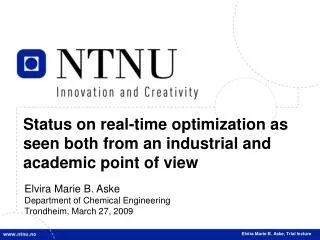
DESIGN OF PLANTWIDE CONTROL SYSTEMS WITH FOCUS ON MAXIMIZING THROUGHPUT. Elvira Marie B. Aske Department of Chemical Engineering Norwegian University of Science and Technology Trondheim, March 27, 2009. Elvira Marie B. Aske, Ph.D. Defense. Presentation outline. Introduction (Chapter 1)

E N D
DESIGN OF PLANTWIDE CONTROL SYSTEMS WITH FOCUS ON MAXIMIZING THROUGHPUT Elvira Marie B. Aske Department of Chemical Engineering Norwegian University of Science and Technology Trondheim, March 27, 2009 Elvira Marie B. Aske, Ph.D. Defense
Presentation outline Introduction (Chapter 1) Self-consistency (Chapter 2) Maximum throughput (Chapter 3 (4,5,6)) Optimal operation Bottleneck Back off Dynamic degrees of freedom for tighter bottleneck control (Chapter 4) Coordinator MPC (Chapter 5,6) Remaining capacity Flow coordination Industrial case Concluding remarks and and further work
Introduction • Optimal economic operation • This often corresponds to maximum throughput • Constrained optimization! • Identifying the constraints? • How does this affect the plantwide control structure? • Frequent disturbances? • Moving constraints?
Chapter 2 Self-consistent inventory control
Self-consistent inventory control • Inventory (material) balance control is an important part of process control • How design an appropriate structure? • Many design rules in literature, but often poor justification • Propose one rule that applies to all cases self-consistency rule
Definitions Consistency: steady-state mass balances (total, component and phase) for the individual units and the overall plant are satisfied. Self-regulation: an acceptable variation in the output variable is achieved without the need for additional control when disturbances occur. Self-consistency: local “self-regulation” of all inventories (local inventory loops are sufficient) Self-consistency is a desired property because the mass balance for each unit is satisfied without the need to rely on control loops outside the unit
Self-consistency rule Rule 2.1. “Self-consistency rule”: Self-consistency (local “self-regulation” of all inventories) requires that • The total inventory (mass) of any part of the process (unit) must be “self-regulated” by its in- or outflows, which implies that at least one flow in or out of any part of the process (unit) must depend on the inventory inside that part of the process (unit). • ... and the inventory of each component • .. and the inventory of each phase
Self-consistency: Example Not “self-regulated”, depends on the other inventory loop OK? Consistent, but not self-consistent
Self-consistency: Example OK? Self-consistent: Interchange the inventory loops
Chapter 3,(4,5 & 6) Maximum throughput
Depending on market conditions: Two main modes of optimal operation Mode 1. Given throughput (“nominal case”) Given feed or product rate “Maximize efficiency”: Unconstrained optimum Mode 2. Max/Optimum throughput Throughput is a degree of freedom + good product prices 2a)Maximum throughput Increase throughput until constraints give infeasible operation Constrained optimum - identify active constraints (bottleneck!) 2b) Optimized throughput Increase throughput until further increase is uneconomical Unconstrained optimum
Throughput manipulator Definition. A throughput manipulator is a degree of freedom that affects the network flows, and which is not indirectly determined by other process requirements. At feed: At product: Inside:
Bottleneck Definition: A unit is a bottleneck if maximum throughput (maximum network flow for the system) is obtained by operating this unit at maximum flow • If the flow for some time is not at its maximum through the bottleneck, then this loss can never be recovered Maximum throughput requires tight control of the bottleneck unit
Back off Definition: The (chosen) back off is the distance between the (optimal) active constraint value (yconstraint) and its set point (ys) (actual steady-state operation point), which is needed to obtain feasible operation in spite of: 1. Dynamic variations in the variable y caused by imperfect control 2. Measurement errors. yconstraint y ys Back off Time
Realize maximum throughput Best result (minimize back-off) if TPM permanently is moved to bottleneck unit Bottleneck (active constraint) = max Note: reconfiguration of inventory loops upstream TPM
Obtaining the back off • Back off given by • Exact estimation of back off difficult in practice • Use controllability analysis to obtain “rule of thumb” • Estimate back off to find economic incentive: • Worst case amplification:
Back off example: PI-control of first order disturbance Frequency response of Sgd Step response in d at t=0
Obtaining the back off (controllability analysis) • “Easy disturbance” • Benefit of control to reduce the peak • Minimum back off: • “Difficult disturbance” • Control gives a larger back off (but needed for set point tracking) • “Smooth” tuning recommended to reduce peak (MS) • Minimum back off:
USE DYNAMIC DEGREES OF FREEDOM Chapter 4
Reduce back off by usingdynamic degrees of freedom • TPM often located at feed (from design) • Not always possible to move TPM • Reconfiguration undesirable (TPM and inventory) • Dynamic reasons (Luyben, 1999) • Alternative solutions: • Use dynamic degrees of freedom (e.g. holdup volumes) • For plants with parallel trains: Use crossover and splits Luyben, W.L. (1999). Inherent dynamic problems with on-demand control structures. Ind. Eng. Chem. Res. 38(6), 2315–2329.
Dynamic degrees of freedom: Main idea • Main idea: change the inventory to make temporary flow rate changes in the units between the TPM (feed) and the bottleneck • Improvement: Tighter bottleneck control, the effective delay from the feed to the bottleneck may be significantly reduced • Cost:Poorer inventory control (usually OK)
Proposed control structure:Single-loop plus ratio control • Change all upstream flows simultaneously • No reconfiguration of inventory loops • Bottleneck control only weakly dependent on inventory controller tuning
Chapter 5 & 6 Coordinator MPCThe approach and the implementation at Kårstø gas plant
Snøhvit Melkøya Kristin Norne Heidrun Åsgard Tjeldbergodden Haltenpipe ÅTS Ormen Lange Statfjord Nyhamna Troll Frigg Kollsnes Vesterled Kårstø Sleipner St Fergus Europipe II Ekofisk Europipe I Langeled Norpipe Zeepipe I Franpipe Dunkerque Easington Emden Zeebrugge North Sea gas network Norwegian continental shelf • Kårstø plant: Receives gas from more than 30 offshore fields • Limited capacity at Kårstø may limit offshore production (both oil and gas) TRONDHEIM Oslo UK GERMANY
Motivation for coordinator MPC: Plant development over 20 years How manipulate feeds and crossovers? Condensate Ethane
Maximum throughput • Here: want maximum throughput Obtain this by “Coordinator MPC”: • Manipulate TPMs (feed valves and crossovers) presently used by operators • Throughput determined at plant-wide level (not by one single unit) coordination required • Frequent changes dynamic model for optimization
”Coordinator MPC”: Coordinates network flows, not MPCs (remaining capacity) Illustration of the coordinator MPC
? Approach Use Coordinator MPC to optimally adjust TPMs: • Coordinates the network flows to the local MPC applications • Decompose the problem (decentralized). • Assume Local MPCs closed when running Coordinator MPC • Need flow network model (No need for a detailed model of the entire plant) • Decoupling: Treat TPMs as DVs in Local MPCs • Use local MPCs to estimate feasible remaining capacity (R) in each unit
Feasible remaining feed capacity for unit k: Obtained by solving “extra” steady-state LP problem in each local MPC: subject to present state, models and constraints in the local MPC Use end predictions for the variables Recalculated at every sample (updated measurements) Very little extra effort! Remaining capacity (using local MPCs) current feed to unit k max feed to unit k within feasible operation
Coordinator MPC: Design Objective: Maximize plant throughput, subject to achieving feasible operation • MVs: TPMs (feeds and crossovers that affect several units) • CVs: total plant feed + constraints: • Constraints (R > backoff > 0, etc.) at highest priority level • Objective function: Total plant feed as CV with high, unreachable set point with lower priority • DVs: feed composition changes, disturbance flows • Model: step-response models obtained from • Calculated steady-state gains (from feed composition) • Plant tests (dynamic)
Kårstø plant Gas processing area Control room
KÅRSTØ MPC COORDINATOR IMPLEMENTATION (2008) Export gas Rich gas MV CV Export gas CV CV CV MV CV CV CV Rich gas CV CV CV MV Half of the plant included: 6 MVs 22 CVs 7 DVs MV CV Condensate MV CV CV MV CV CV CV CV CV
Step response models in coodinator MPC Remaining capacity (R) goes down when feed increases… + more…
Experiences • Using local MPCs to estimate feasible remaining capacity leads to a plant-wide application with “reasonable” size • The estimate remaining capacity relies on • accuracy of the steady-state models • correct and reasonable CV and MV constraints • use of gain scheduling to cope with larger nonlinearities (differential pressures) • Crucial to inspect the models and tuning of the local applications in a systematic manner • Requires follow-up work and extensive training of operators and operator managers • “New way of thinking” • New operator handle instead of feed rate: Rs (back-off)
Main contributions • Plantwide decomposition by estimating the remaining capacity in each unit by using the local MPCs • The idea of using a “decentralized” coordinator MPC to maximize throughput • The proposed self-consistency rule, one rule that applies to all cases to check whether a inventory control system is consistent • Single-loop with ratio control as an alternative structure to obtain tight bottleneck control
Further work • Recycle systems not treated • Information loss in plantwide composition • Further implementation of coordinator MPC • Planned start-up autumn 2009 (after control system upgrade) • Acknowledgments: Gassco, StatoilHydro ASA