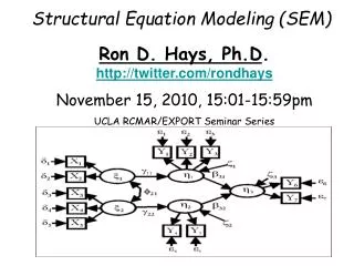
Stages in Structural Equation Modeling
Stages in Structural Equation Modeling. The Stages in Structural Equation Model. Stage 1) Assessing individual constructs Stage 2) Developing and assessing the measurement model validity Stage 3) Specifying the structural model Stage 4) Assessing structural model validity.

Stages in Structural Equation Modeling
E N D
Presentation Transcript
The Stages in Structural Equation Model • Stage 1) Assessing individual constructs • Stage 2) Developing and assessing the measurement model validity • Stage 3) Specifying the structural model • Stage 4) Assessing structural model validity
Stage 1:Assessing Individual constructs • One of the most important steps is operationalization of constructs (Hair, 2006). • In attempting to ensure theoretical accuracy, researchers many times have a number of established scales to choose from. Nonetheless, eve with the wide usage of scales, the researcher often is faced with the lack of an established scale and must develop a new scale or substantially modify an existing scale to new context. • Therefore, in all of these conditions, the foundation for the SEM analysis is how selects the items to measure the constructs (Hair et al., 2006).
Type of Individual construct Type2: Individual Construct with 3 dimension First –Order CFA Type1: Simple Individual Construct Type3: Construct with 3 dimension based on Second –Order CFA
Single factor Independent Model Interrelated model
Goodness-of-Fit Criteria • Goodness-of-Fit measures can be classified into three types (Ho, 2006): • Absolute fit measures: These measures determine the degree to which the proposed model predicts (Fits) the observed covariance matrix. Some commonly used measures of absolute fit such as: a) Chi-square: In SEM, the researcher is looking for significant differences between the actual and predicted matrices. As such, the researcher does not wish to reject the null hypothesis and, accordingly, thesmallerthe chi-square value, the better fit of the model. b) Normed Chi-square/df: Values close to 1.0 indicate good fit. values between 2.0 and 3.0 indicate reasonable fit. c) Goodness-of-Fit Index(GFI): value> 0.90 d) Root Mean Square Error of Approximation(RMSEA); Hair, et al., (2006; p748) recommended RAMSEA between .03 and .08. Kline (2011, p 206 and 2005, p139) RAMSEA < .05 indicates close approximate fit, between .05 and .08 reasonable, and RAMSEA > .10 suggest poor fit (cited from Browne & Cudek, 1993) -e) Standardised Root Mean-square Residual (SRMR): values less than .10 are generally considered favorable (Kline, 2005, p141)
Goodness-of-Fit Criteria (2) Incremental fit measures: These measures compare the proposed model to some baseline model, most often referred to as the null or independence model. In the independence model, the observed variables are assumed to be uncorrelated with each other. Incremental fit measures have been proposed, such as: -Tucker-Lewis Index (TLI)-Normed Fit Index (NFI) -Relative Fit Index (RFI) -Incremental Fit Index (IFI) -Comparative Fit Index (CFI) • By convention, researchers have used incremental fit indices > 0.90 as traditional cutoff values to indicate acceptable levels of model fit. the model represents more than 90% improvement over the null or independence model. In other words, the only possible improvement to the model is less than 10%.
Goodness-of-Fit Criteria (3) Parsimonious fit measures:In scientific research, theories should be as simple, or parsimonious, as possible (Ho, 2006). parsimonious fit measures relate the goodness-of-fit of the proposed model to the number of estimated coefficients required to achieve this level of fit. Such as: • Parsimonious Normed Fit Index (PNFI): When comparing between models, differences of 0.06 to 0.09 are proposed to be indicative of substantial model differences (Williams & Holahan, 1994). • Akaike Information Criterion (AIC): The AIC is a comparative measure between models with differing numbers of constructs. AIC values closer to zero indicate better fit and greater parsimony. A small AIC generally occurs when small chi-square values are achieved with fewer estimated coefficients.
Detecting outliers • The Mahalanobis D2 statistics is commonly used to detect case-wise outliers. It computes the overall centroid and computes the distance of each observation from the centroid. • The Mahalanobis D2 is known to follow a Chi-square distribution. The degree of freedom is the number of variables that are being tested. • Usually the inverse chi-square value at a=0.001 is taken as the trash hold value. • For example there are 2 variables, then df=2 • Inverse Chi-squared value for a=0.001 at a df of 2 is: 13.186 • If the highest value in the MAH_1 column is 6.784, which is less than 13.186. Thus, there are no major outliers in the file.
different method to handle missing values • Listwise deletion: means a subject with missing values is deleted in all calculations. • Pairwise: means it is deleted subjects with missing data just for calculations comprising that variable. In using the Listwise deletion and Pairwise deletion may be losing a large number of cases, and then could reduce the sample size, therefore these two methods are not always suggested (Schumacher & Lomax, 2010). • The SEM softwaresthe option for handling the missing values are replacing the missing value with means when only a small number of missing values is present in the data set, or employed regression imputations for handle missing values when a moderate amount of missing data present in the data (Schumacher & Lomax, 2010; Byrne, 2010).
Examples and hands on For Individual construct CFA
Stage 2) Developing and assessing the measurement model validity • While specified the scale items, it is essential to specify the measurement model. In this stage, each latent construct to be included in the model is identified and the measured indicator variables (items) are assigned to latent constructs (Hair et al., 2006). • The measurement models specify how the latent variables are measured in terms of the observed variables. In the other word the measurement models are concerned with the relations between observed and latent variables (Ho, 2006).
The Criteria's for Assessment Goodness-Of-Fit (GOF) Indices • Assessing the individual constructs, measurement model validity and structural model validity depends on a number of Goodness-Of-Fit (GOF) indices • Goodness-of-fit measures the extent to which the actual or observed covariance input matrix corresponds with (or departs from) that predicted from the proposed model (Ho, 2006). • GOF measures such as : Chi-Square (non sig), Goodness of Fit Indicator (GFI), Adjusted Goodness of Fit Indicator (AGFI), Comparative Fit Index (CFI), Normed Fit Index (NFI), and Tucker Lewis Index (TLI) indicates a good fit to the model at about .9 or greater. Root Mean Square Error of Approximation (RMSEA) which a measure greater than .1 indicates a poor fit, values ranging between 0.08 to 0.1 indicate mediocre fit, and values ranging between 0.03 and 0.08 are indicate better fit model.
The Criteria's for Assessment Construct validity Construct validity is the extent to which a set of measured items actually reflected the theoretical latent construct those item are designed to measure. Thus, it deals with the accuracy of measurement. Construct validity is made up of four important components which they are: 1) Convergent validity: the items that are indicators of a specific construct should converge or share a high proportion of variance in common, known as convergent validity. The ways to estimate the relative amount of convergent validity among item measures: Factor Loading: at a minimum, all factor loading should be statistically significant. A good rule of thumb is that standardized loading estimates should be .5 or higher, and ideally .7 or higher. Variance Extracted (VE): is the average squared factor loading. A VE of .5 or higher is a good rule of thumb suggesting adequate convergence. A VE less than .5 indicates that on average, more error remains in the items than variance explained by the latent factor structure impose on the measure (Haire et al., 2006, p 777). Construct Reliability: construct reliability should be .7 or higher to indicate adequate convergence or internal consistency.
The Criteria's for Assessment Construct validity 2) Discriminant Validity: the extent to which a construct is truly distinct frame other construct. To test the discriminant validity the VE for two factors should be grater than the square of the correlation between the two factors to provide evidence of discriminant validity. 3) Nomological Validity: is tested by examining wheather the correlation among the constructs in a measurement theory make sense. Constructs of interest should be related to other constructs according to hypothesised ways derived from the theory in which the construct is embeded, forming the nomological net for that set of constructs (The matrix of correlations can be useful in this assessment. 4) Face Validity: must be established prior to any theoretical testing when using CFA. Without an understanding of every item’s content or meaning. It is impossible to express an correctly specify a measurement theory.
Stage 3)Specifying the structural model • Once the measurement model is specified and validated with CFA, then the structural model represented by specifying the set of relationships between constructs. • The structural equation model is a comprehensive model that specifies the pattern of relationships among independent and dependent variables, either observed or latent (Hair, et al., 2010; Ho, 2006; Landis et al., 2001).
Stage 4) Assessing structural model validity • The assessing structural model validity focused on two issues comprising; • a) the overall and relative model fit, and • b) the size, direction, and significance of the structural parameter estimates, depicted with one-headed arrows on a path diagram (Hair et al., 2006).
Accounting for Error • Thus, SEM provides estimates for two types of error variance – error terms and residual terms: • Error term: represents measurement error associated with observed variables, i.e. the degree to which the observed variables do not perfectly describe the latent construct of interest (Hair, Black et al. 2006). Such measurement error terms represent causes of variance due to unmeasured variables as well as random measurement error (Garson 2006). • Residual term: represents the error in the prediction of endogenous factors from exogenous factors, that is to say, how much variance in the associated endogenous variable was not accounted for by influences in the model (Texas 2002).
Approaches to aggregation • Total disaggregation: In a totally disaggregated model, each item serves as an indicator for a construct. • Partial disaggregation: In a partially disaggregated model, several items are summed or averaged resulting in parcels. These parcels are then used as indicators for constructs. • Total aggregation: In a totally aggregated model, all of the items for a scale are summed or averaged. The result is that if only one scale is used to measure each construct, then there is only one indicator per construct and the model is a path analysis rather than a latent variable model. If more than one scale was used to measure a construct, then it is still possible to specify a latent variable, and each indicator is a total scale score (Coffman and Maccall.um, 2005).
Parceling • Parcels are aggregations (sums or averages) of several individual items. • Advantages of parcels (Coffman and Maccall.um, 2005) : • parcels generally have higher reliability than single items(Kishton & W idaman, 1994). • A second advantage of using parcels rather than items as indicators of latent variables involves the reduction in the number of measured variables in a model. From this perspective, models with parcels as indicators are likely to fit better than models with items as indicators because the order of the parcel correlation matrix is much smaller than the order of the item correlation matrix. • They can be used as an alternative to data transformations or alternative estimation techniques when working with nonnormally distributed variables. The most often used estimation method in structural equation modeling, maximum likelihood, assumes multivariate normality of the measured variables in the population. If the measured variables are not multivariate normal, then estimates of fit measures and estimates of standard errors of parameters may not be accurate (Hu & Bentler, 1998).