The Problem with Integer Programming
The Problem with Integer Programming. H.P.Williams London School of Economics. The Nature of Integer Programming (IP). Is IP like Linear Programming (LP) ? Applications of Integer Programming Mathematical Properties of IP Economic Properties of IP Chv á tal Functions and Integer Monoids.

The Problem with Integer Programming
E N D
Presentation Transcript
The Problem with Integer Programming H.P.Williams London School of Economics
The Nature of Integer Programming (IP) • Is IP like Linear Programming (LP) ? • Applications of Integer Programming • Mathematical Properties of IP • Economic Properties of IP • Chvátal Functions and Integer Monoids
A General (Mixed) Integer Programme (IP) Maximise/Minimise ∑j cjxj+∑kdkyk Subject to:∑jaijxj +∑keikyk <=> bi for all i xj>=0 all j, yk>=0 all k and integer
A General (Mixed) Integer Programme • Frequently (but not always) the integer variables are restricted to values 0 and 1 representing (indivisible) Yes/No decisions eg. Investment • Can view as a Logicalstatement about a series of Linear Programmes (LPs) • Leads a to close relationship between Logic and IP
0-1 Integer Programmes • Any IP with bounded integer variables can be converted to a 0-1 IP • 0-1 IPs can be interpreted as Disjunctions ofLPs • Application of logical methods to formulation and solution
Applications of IP • Extensions to LPs eg Manufacturing, Distribution, Petroleum, Gas and Chemicals • Global Optimisation of non-convex (non-linear) models • Power Systems Loading • Facilities Location • Routing • Telecommunications • Medical Radiation • Statistical Design • Molecular Biology • Genome Sequencing • Archaeological Seriation • Optimal Logical Statements • Computer Design • Aircraft Scheduling • Crew Rostering
Linear Programming v Integer Programming An LP Minimise X2 Subject to: 2X1+X2 >=13 5X1+2X2<=30 -X1+X2 >=5 X1 , X2 >= 0 The Solution • X1 = 22/3 , X2 = 72/3
Linear Programming v Integer Programming An LP Minimise X2 Subject to: 2X1+X2 >=13 5X1+2X2<=30 -X1+X2 >=5 X1 , X2 >= 0 The Solution • X1 = 22/3 , X2 = 72/3 An IP Minimise X2 Subject to: 2X1 + X2 >=13 5X1 + 2X2<=30 -X1 + X2 >=5 X1 , X2 >= 0 and integer
Linear Programming v Integer Programming An LP Minimise X2 Subject to: 2X1+X2 >=13 5X1+2X2<=30 -X1+X2 >=5 X1 , X2 >= 0 The Solution • X1 = 22/3 , X2 = 72/3 The Solution • X1 = 2 , X2 = 9 An IP Minimise X2 Subject to: 2X1 + X2 >=13 5X1 + 2X2<=30 -X1 + X2 >=5 X1 , X2 >= 0 and integer
LP and IP Solutions 9 . . . . . Min x2 c3st 2x1+ x2 >= 13 8 . . c1 . . 5x1 + 2x2 <= 30 x2 -x1 + x2 >= 5 7 . . . . c2 . x1 , x2 >= 0 6 . . . . . 5 . . . . . 0 1 2 3 4 x1
LP and IP Solutions 9 Optimal IP Solution (2 , 9).Min x2 c3st 2x1+ x2 >= 13 8 . . c1 . . 5x1 + 2x2 <= 30 Optimal LP Solution (2 2/3 , 7 2/3) -x1 + x2 >= 5 7 . . . . c2 . x1 , x2 >= 0 x2 6 . . . . . 5 . . . . . 0 1 2 3 4 x1 •
IP Solution after removing constraint 1 Min x2 8 c1 . . . c3 st5x1 + 2x2 <= 30 -x1 + x2 >= 5 . . . . x1 , x2 >= 0 x27 . . . 6 . . . . . c2 Optimal IP Solution (0 , 5) 5 0 1 2 3 4 x1 •
IP Solution 9 Optimal IP Solution (2 , 9).Min x2 c3st 2x1+ x2 >= 13 8 . . c1 . . 5x1 + 2x2 <= 30 Optimal LP Solution (2 2/3 , 7 2/3) -x1 + x2 >= 5 7 . . . . c2 . x1 , x2 >= 0 x2 6 . . . . . 5 . . . . . 0 1 2 3 4 x1 •
IP Solution after removing constraint 2 9 . . . Min x2 c1 c3 st 2x1+ x2 >= 13 8 . . . .Optimal IP Solution (3, 8) -x1 + x2 >= 5 7 . . . . . x1 , x2 >= 0 x2 6 . . . . . 5 . . . . . x1 0 1 2 3 4 •
IP Solution 9 Optimal IP Solution (2 , 9).Min x2 c3st 2x1+ x2 >= 13 8 . . c1 . . 5x1 + 2x2 <= 30 Optimal LP Solution (2 2/3 , 7 2/3) -x1 + x2 >= 5 7 . . . . c2 . x1 , x2 >= 0 x2 6 . . . . . 5 . . . . . x1 0 1 2 3 4 •
IP Solution after removing constraint 3 9 . . . . Min x2 st 2x1+ x2 >= 13 8 . . . . . 5x1 + 2x2 <= 30 c1 c2 x1 , x2 >= 0 7 . . . . . x2 6 . . . . . 5 . . . . .Optimal IP Solution (4 , 5) 0 1 2 3 4 x1
Rounding often not satisfactoryExample: The Alabama Paradox • State Population Fair solution Rounded Solution With 10 Representatives A 621k 4.41 4 B 587k 4.17 4 C 201k 1.43 2 With 11 Representatives A 621k 4.85 5 B 587k 4.58 5 C 201k 1.57 1
IP Formulation of Political Apportionment Problem Vi = Population (Votes cast) for State (Party) i xi = Seats allotted to State (Party) i Choose xi so as to: Min Maxi (xi / vi) st ∑ixi = Total Number of Seats xi >= 0 and integer for all I ie Min y st xi / vi <= y for all i ∑i xi = Total Number of Seats xi >= 0 and integer for all I LP Relaxation gives fractional solution IP Solution give Jefferson/D’Hondt solution
IP Solution • State Population Fractional Rounded Jefferson/ solution solution D’Hondt solution (LP) (IP) With 10 Representatives A 621k 4.41 4 5 B 587k 4.17 4 4 C 201k 1.43 2 1 With 11 Representatives A 621k 4.85 5 5 B 587k 4.58 5 5 C 201k 1.57 1 1
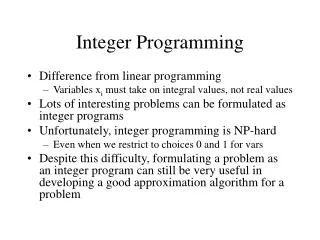
Mathematical Differences between LP and IP • Consider a (Pure) IP in standard form Maximise c1x1+ c2x2 + … + cnxn Subject to: a11x1 + a12x2 + … a1nxn <= b1 a21x1 + a22x2 + … a2nxn <= b2 . . am1x1+ am2x2 + … amnxn <= bm x1 , x2 , … , xn >= 0 and integer
Mathematical Differences between LP and IP • LP IP If has Optimal Solution No limit on number of positive variables there is one with at most m variables positive (a basic solution) Hilbert Basis (no fixed dimension) At most nconstraints At most 2n– 1 binding at optimum constraints binding at optimum There are valuations Chvátal Functions on constraints which close duality gap ie there is a (symmetric) LP No obvious symmetry (dual) model
IPs involve Lattices within Polytopes Eg Max 2x1+x2 st 2x1+9x2<=80 2x1-3x2<=6 -x1 <=0 -x2<=0 2x1+3x2 ≡0(mod12) x1 ≡0(mod1) x2≡0(mod1)
What are the strongest implications? Max 2x1+x2 st 2x1+9x2<=80 2x1+9x2<=80 2x1-3x2<=6 2x1-3x2<=6 -x1 <=0 -x1 <=0 2x1+x2 ? -x2<=0 -x2<=0 2x1+3x2 ≡0(mod12) 2x1+3x2 ≡0(mod12) x1 ≡0(mod1) x1 ≡0(mod1) 2x1+x2 ? x2≡0(mod1) x2 ≡0(mod1)
What are the strongest implications? Dual arguments. Max 2x1+x2 st 2x1+9x2<=80 2x1+9x2<=80⅓ 2x1-3x2<=6 2x1-3x2<=6⅔ -x1 <=0 -x1 <=002x1+x2 <= 302/3 -x2<=0 -x2<=00 2x1+3x2 ≡0(mod12) 2x1+3x2 ≡0(mod12)3 x1 ≡0(mod1) x1 ≡0(mod1)02x1+x2 Ξ0(mod4) x2≡0(mod1) x2 ≡0(mod1)4
IPs involve Lattices within Polytopes 8.. . ..Objective = 302/3 4.. . Objective = 28 . . . . . Objective = 24 0 6 12
IPs involve Lattices within Polytopes Optimisation over polytopes give strongest (LP) bound on objective Optimisation over lattices give strongest congruence relation for objective Combined they give rank 1 cut for objective This may not be adequate
Lattices within Cones give Integer Monoids These are a fundamental structure for IP
Polyhedral and Non-Polyhedral Monoids The integer lattice within the polytope -2x + 7y >= 0 x – 3y >= 0 A Polyhedral Monoid y 4 . . . . . . . . . . . . . . . 3 . . . . . . . . . .. . . . . 2 . . . . . . .. . . . . . . . 1 . . . . . . . . . . . . . . . ……. 0. . . . . . . . . . . . . . . 0 1 2 3 4 5 6 7 8 9 10 11 12 13 14 x Projection: A non-polyhedral monoid (Generators 3 and 7) x .. x .. x x . x x. x x x…….
Polyhedral and Non-Polyhedral Monoids 4 . . . . . . . . . . . . . . . 3 . . . . . . . . . .. . . . . 2 . . . . . . .. . . . . . . . 1 . . . . . . . . . . . . . . . ……. 0. . . . . . . . . . . . . . . 0 1 2 3 4 5 6 7 8 9 10 11 12 13 14 x Projection: A non-polyhedral monoid (Generators 3 and 7) x.. x .. x x. x x. x x x……. Reverse Head 11 10 9 8 7 6 5 4 3 2 1 0 . x x . x x .. x .. x
Duality in LP and IP The Value Function of an LP Minimise x2 subject to: 2x1 + x2 >= b1 5x1 + 2x2 <= b2 -x1 + x2 >= b3 x1 , x2 >= 0 Value Function of LP is Max(5b1 -2b2 , 1/3( b1 + 2b3) , b3) If b1 = 13, b2 = 30, b3 = 5we have Max( 5, 72/3 , 5 ) = 72/3 , Consistency Tester is Max(2b1 – b2 , -b2 , -b2 + 2b3 ) <= 0 giving Max( -4, -30, -20) <= 0 . (5, -2, 0), (1/3, 0, 2/3), (0, 0, 1) are vertices of Dual Polytope . They give marginal rates of change (shadow prices) of optimal objective with respect to b1, b2, b3 . (5, -2,, 0), (1/3, 0, 2/3), (0, 0, 1) are extreme rays of Dual Polytope . What are the corresponding quantities for an IP ?
LP Solution 9 . . . . Min x2 c3st 2x1+ x2 >= 13 8 . . c1 . . 5x1 + 2x2 <= 30 Optimal LP Solution (2 2/3 , 7 2/3) -x1 + x2 >= 5 7 . . . . c2 . x1 , x2 >= 0 x2 6 . . . . . 5 . . . . . 0 1 2 3 4 x1
IP Solution 9 Optimal IP Solution (2 , 9). . . Min x2 c3st 2x1+ x2 >= 13 8 . . c1 . . 5x1 + 2x2 <= 30 Optimal LP Solution (2 2/3 , 7 2/3) -x1 + x2 >= 5 7 . . . . c2 . x1 , x2 >= 0 x2 6 . . . . . 5 . . . . . 0 1 2 3 4 x1
Duality in LP and IP The Value Function of an IP Minimise x2 subject to: 2x1 + x2 >= b1 5x1 + 2x2 <= b2 -x1 + x2 >= b3 x1 , x2 >= 0 and integer Value Function of IP is Max( 5b1 -2b2 ,┌1/3( b1 + 2b3) ┐ , b3 , b1+ 2 ┌ 1/5 (-b2+ 2┌1/3(b1 + 2b3) ┐ ) ┐ ) This is known as a Gomory Function. The component expressions are known as Chvάtal Functions . Consistency Tester same as for LP (in this example)
Gomory and Chvátal Functions Max( 5b1-2b2, ┌1/3(b1 + 2b3) ┐, b3 , b1+ 2 ┌1/5 (-b2+ 2┌1/3(b1 + 2b3) ┐ ) ┐ ) If b1=13, b2=30, b3=5 we have Max(5,8,5,9)=9 Chvátal Function b1+ 2 ┌1/5 (-b2+ 2┌1/3(b1 + 2b3) ┐ )┐determines the optimum. LP Relaxation is 19/15 b1 - 2/5 b2 +8/15 b2 (19/15, -2/5, 8/15) is an interior point of dual polytope but (5, -2, 0) and (1/3, 0, 2/3) are vertices of dual corresponding to possible LP optima (for different bi )
Why are valuations on discrete resources of interest ? Allocation of Fixed Costs Maximise ∑j pi xi - f y stxi - Di y<= 0 for all I y ε {0,1} depending on whether facility built. f is fixed cost. xi is level of service provided to i (up to level Di ) pi is unit profit to i. A ‘dual value’ vion xi - Di y<= 0 would result in Maximise ∑j (pi – vi ) xi - (f – (∑j D i v i) y Ie an allocation of the fixed cost back to the ‘consumers’
A Representation for Chvátal Functions b1 b3 -b2 1 2 Multiply and add on arcs 1 1 Divide and round up on nodes 2 2 Giving b1+ 2 ┌1/5( -b2+ 2┌1/3( b1 + 2b3) ┐ ) ┐ LP Relaxation is19/15 b1 - 2/5 b2 +8/15 b3 3 5 1
Simplifications sometimes possible • ┌ 2/7 ┌7/3n┐┐ ≡ ┌2/3n┐ • But ┌ 7/3 ┌2/7n┐┐ ≠ ┌2/3n┐ eg n = 1 • ┌ 1/3 ┌ 5/6n┐┐ ≡ ┌5/18n┐ • But ┌ 2/3 ┌ 5/6n┐┐ ≠ ┌5/9n┐ eg n = 5 Is there a Normal Form ?
Properties of Chvátal Functions • They involve non-negative linear combinations (with possibly negative coefficients on the arguments) and nested integer round-up. • They obey the triangle inequality. • They are shift-periodic ie value is increased in cyclic pattern with increases in value of arguments. • They take the place of inequalities to define non-polyhedral integer monoids.
The Triangle Inequality • ┌a┐ + ┌b┐ >= ┌a + b┐ • Hence of value in defining Discrete Metrics
A Shift Periodic Chvátal Function of one argument ┌ ½ ( x + 3 ┌ x /9 ┐ ) ┐ is (9, 6) Shift Periodic. 2/3is ‘long-run marginal value’ 14 13 12 11 10 9 8 7 6 5 4 3 2 1 . 0 1 2 3 4 5 6 7 8 9 10 11 12 13 14 15 16 17 18 19 20 21 22 23 24 25 26 27 28 29 30 --- x
Polyhedral and Non-Polyhedral Monoids The integer lattice within the polytope -2x + 7y >= 0 x – 3y >= 0 A Polyhedral Monoid 4 . . . . . . . . . . . . . . . 3 . . . . . . . . . .. . . . . 2 . . . . . . .. . . . . . . . 1 . . . . . . . . . . . . . . . ……. 0. . . . . . . . . . . . . . . 0 1 2 3 4 5 6 7 8 9 10 11 12 13 14 Projection: A Non-Polyhedral Monoid (Generators 3 and 7) x .. x .. x x . x x . x x x ……. Defined by ┌-x /3┐ +┌2x /7┐ < = 0
Finally • We should be Optimising Chvátal Functions over Integer Monoids
References • CE Blair and RG Jeroslow, The value function of an integerprogramme, Mathematical Programming 23(1982) 237-273. • V Chvátal, Edmonds polytopes and a hierarchy of combinatorialproblems, Discrete Mathematics 4(1973) 305-307. • D.Kirby and HP Williams, Representing integral monoids by inequalities Journal of Combinatorial Mathematicsand Combinatorial Computing 23 (1997) 87-95. • F Rhodes and HP Williams Discrete subadditive functions as Gomory functions, Mathematical Proceedings of the CambridgePhilosophicalSociety 117 (1995) 559-574. • HP Williams, A Duality Theorem for Linear Congruences, Discrete Applied Mathematics 7 (1984) 93-103. • HP Williams, Constructing the value function for an integer linear programme over a cone, Computational Optimisation andApplications 6 (1996) 15-26. • LA Wolsey, The b-hull of an integer programme, Discrete Applied Mathematics 3(1981) 193-201.