Download
1 / 17
170 likes | 273 Vues
This lecture covers the principles of active filters, specifically focusing on series and parallel combinations. Students are advised to read Chapter 15.4 and complete related problems as practice. Essential topics include operational amplifiers (Op Amps), feedback mechanisms, initial conditions, and voltage gain calculations. The lecture also explores differentiators and low-pass filter characteristics. A quiz will assess comprehension, with emphasis on topics from Chapters 14 and 15. Details on filter behavior and phase relationships are addressed, enhancing understanding of complex circuit functions.

E N D
ECEN3713 Network AnalysisLecture #21 28 March 2006Dr. George Scheets • Read Chapter 15.4 • Problems: 13.78, 15.5 – 15.7 • Thursday's Quiz • Series or Parallel Combinations of Active Filters Thursday's Assignment Problems 15.8, 15.10, 15.11, 15.20 Quiz 7 kicked back for a regrade.
ECEN3713 Network AnalysisLecture #23 4 April 2006Dr. George Scheets • Read Chapter 15.5 - End of Chapter • Problems: 15.21, 15.22, 15.24, 15.25 • Test on Thursday!Focus is on Material after last test • Chapters 14 & 15 • Initial Conditions • Chapters 12 & 13 may also show up
Op Amp Characteristics +Vcc vp(t) Av Zin + • Zin? • In M ohms • Hopamp(f) f3dB? • In XX or XXX MHz • Voltage gain Av? • On order of 104 - 106 vout(t) = Av(vp(t)-vn(t)) vn(t) - -Vcc
Op Amps: No Feedback +Vcc • Output likely to hit rails • Unless tiny voltages Av + vout(t) = Av(vp(t)-vn(t)) vin(t) - -Vcc
Op Amps: Positive Feedback • Output likely to hit rails • May get stuck there Av vout(t) + vin(t) -
Op Amps: Negative Feedback • Safe to assume vp(t) = vn(t) • Safe to assume no current enters Op Amp • If low Z outside paths exist Av vout(t) - 0 v vin(t) +
Op Amps: Output Load • Ideally, load does not effect characteristics • Practically, load may effect characteristics • If Op Amp output can't source or sink enough current Av vout(t) - vin(t) + Zload
Differentiator: H(jω) = -jωRC |H(ω)| 1 ω 0 100 1000
5 Hz Square Wave In... 1.5 0 -1.5 1.0 0 This curve made up of 100 sinusoids. Fundamental frequency of 5 Hz & next 99 harmonics (15, 25, ..., 995 Hz).
Spikes Out... 1.5 0 -1.5 1.0 0
1st Order RC Low Pass Filter |H(ω)| 1 0.707 1 ω
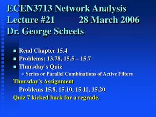
2nd Order Low Pass Filter(Two back-to-back 1st order active filters) |H(ω)| 3dB break point changes. 1 0.707 1st order 2nd order 1 ω
Scaled 2nd Order Low Pass Filter(Two back-to-back 1st order active filters) |H(ω)| 2nd order filter has faster roll-off. 1 0.707 1st order 2nd order 1 ω
2nd Order Butterworth Filter |H(ω)| Butterworth has flatter passband. 1 0.707 2nd order Butterworth 2nd order Standard 1 ω
1 & 2 Hz sinusoids1000 samples = 1 second 1.5 i 0 x1 i - 1.5 samples 0 200 400 600 800 1000 0 i 3 1 ´ 10 Suppose we need to maintain a phase relationship (low frequency sinusoid positive slope zero crossing same as the high frequency sinusoid's).
1 & 2 Hz sinusoids1000 samples = 1 secondBoth delayed by 30 degrees 1.5 0 - 1.5 0 200 400 600 800 1000 0 i 3 1 ´ 10 Delaying the two curves by the same phase angle loses the relationship.
1.5 0 - 1.5 0 200 400 600 800 1000 0 i 3 1 ´ 10 1 & 2 Hz sinusoids1000 samples = 1 second1 Hz delayed by 30, 2 Hz by 60 degrees Delaying the two curves by the same time keeps the relationship. θlow/freqlow needs to = θhi/freqhi. A transfer function with a linear phase plot θout(f) = Kθin(f) will maintain the proper relationship.