
Quick Guide to TCUI in mrVista: Analyzing Time Courses for ROI
This guide provides a concise overview of the TCUI (Time Course User Interface) within the mrVista software, designed for performing basic analyses on time courses across multiple scans for a specified Region of Interest (ROI). It details the requirements for analyzing cyclic and event-related data, outlining various plotting options available, including whole time courses, mean time courses, and relative amplitudes. Ideal for researchers looking to visualize and interpret fMRI data efficiently.

Quick Guide to TCUI in mrVista: Analyzing Time Courses for ROI
E N D
Presentation Transcript
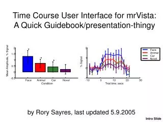
Intro Slide 2 2 * Face Animal 1.5 Car * 1 Novel 1 * Mean Amplitude, % Signal % Signal 0.5 0 0 -0.5 -1 Face Animal Car Novel -10 0 10 20 30 Condition Trial time, secs Time Course User Interface for mrVista: A Quick Guidebook/presentation-thingy by Rory Sayres, last updated 5.9.2005
What’s The TCUI For? What’s It For? The Interface is used to easily view and perform basic analyses on time courses across many scans for a given ROI. It can be used on cyclic (conditions cycle through—e.g., ABAB, traveling-wave) or event-related (including block experiments where the block order is not cyclic) data. What Do You Need? A stim/parfiles directory within your mrVista session directory. If you’re using event-related data, you’ll need .par files in this directory specifying the onset times of different types of trials for each scan. The format is this: ASCII text file w/ two columns; first column is onset time in seconds of a trial, second column is an integer specifying the condition number of that trial. Use 0 to denote null or baseline-condition trials. An optional third column can be used to specify a text label for each condition. Only the label for the first trial for each condition is used. For cyclic data, the .par files can be generated automatically when the TCUI is invoked.
Plotting Options Plotting Options: 1) Whole Time Course: show the time series for the selected ROI from all selected scans, indicating the start of different trials. 2) Mean Time Course: Plot the Mean time course +/- SEMs for each selected condition in the same axes. 3) Mean Time Course Subplots: Plot the mean +/- SEMs for each selected condition in a separate subplot. 4) All Trials: For each condition, plot the peri-stimulus time course from all trials in a separate subplot. 5) Relative Amplitudes: Plot the “dot-product” relative fMRI amplitude for each condition (described below). 6) Mean Amplitudes: Plot the mean difference between BOLD signal between designated “peak” and “baseline” periods (described below). 7)Mean Time Course Plus Amplitudes: Plot the mean amplitudes (option 5) and mean time courses (option 3) together. The default option. 8) FFT of mean tSeries: Perform a Fast Fourier Transform analysis on the mean time series across scans, and plot the results, labeling the frequency at which most events occur in the scans. 9) GLM: Apply a general linear model to the time series and illustrate the results.
Plot Whole Timecourse (1) 2 Face Animal 1.5 Car 1 Novel 0.5 % Signal 0 -0.5 -1 -1.5 20 40 60 80 100 120 140 160 180 200 Time, secs 1) Whole Time Course: show the time series for the selected ROI from all selected scans, indicating the start of different trials. The black periods are baseline periods (condition 0), the other colors reflect the extend of different trial types. The detrended time series is shown in white, in units of % signal change (from either the mean of the raw time series [default] or the mean during the null condition—see Settings).
Plot Whole Timecourse (2) 1) Whole Time Course: show the time series for the selected ROI from all selected scans, indicating the start of different trials. If the length of the whole time series is more than 200 seconds, a slider appears allowing you to navigate through the scan at a reasonable zoom. The “WholeTC” button allows you to zoom out and see the whole time course at once. You can also selectView | Figure Toolbar, and select the zoom icon, to zoom arbitrarily.
Plot Mean Timecourse 2 Face Animal Car 1.5 Novel 1 % Signal 0.5 0 -0.5 -1 -10 -5 0 5 10 15 20 25 Trial time, secs 2) Mean Time Course: Plot the Mean time course +/- SEMs for each selected condition in the same axes.
Plot Mean Tc Subplots Face Car * * 1.5 1.5 1 1 % Signal 0.5 0.5 0 0 -0.5 -0.5 -5 0 5 10 15 20 -5 0 5 10 15 20 Animal Novel * 1.5 1.5 1 1 % Signal 0.5 0.5 0 0 -0.5 -0.5 -5 0 5 10 15 20 -5 0 5 10 15 20 Trial time, secs Trial time, secs 3) Mean Time Course Subplots: Plot the mean +/- SEMs for each selected condition in a separate subplot. This may be more useful if there are many conditions or the amplitude of response is similar for some conditions.
Plot All Trials (1) Face Car * * 2 2 1 1 % Signal 0 0 -1 -1 -5 0 5 10 15 20 -5 0 5 10 15 20 Animal Novel * 2 2 1 1 % Signal 0 0 -1 -1 -5 0 5 10 15 20 -5 0 5 10 15 20 Trial time, secs Trial time, secs 4) All Trials: For each condition, plot the peri-stimulus time course from all trials in a separate subplot. Each trace is a separate trial, relative to the trial onset. If the “Show legend” setting is off, the traces are color coded by condition type…
Plot All Trials (2) Face Car * * 1 2 2 2 3 1 1 % Signal 4 0 0 Trial # -1 -1 -5 0 5 10 15 20 -5 0 5 10 15 20 Animal Novel * 2 2 1 1 % Signal 0 0 -1 -1 -5 0 5 10 15 20 -5 0 5 10 15 20 Trial time, secs Trial time, secs 4) All Trials: For each condition, plot the peri-stimulus time course from all trials in a separate subplot. …if the legend is on, the traces are color-coded by the occurrence of each trial in the whole time series (more blue==occurred earlier, more green==occurred later).
Plot Relative Amplitudes 1.6 Face Animal 1.4 Car 1.2 Novel 1 0.8 Relative amplitude 0.6 0.4 0.2 0 -0.2 Face Animal Car Novel 5) Relative Amplitudes: Plot the “dot-product” relative fMRI amplitude for each condition (described below).
What Are Relative Amplitudes? What are relative amplitudes and how are they computed? We use the metric adopted in (Ress & Heeger, Nat Neurosci 2000). The following steps are taken: 1) All trials are set to have a mean of 0 % signal. (This doesn't affect future plotting, if for example 0% is set as the null condition). 2) The mean time course across all selected trials is computed. 3) For each trial, the dot product between that trial's time course and the mean time course is computed. This gives oneamplitude for each trial. 4) The mean +/- SEM of these amplitudes are plotted for each condition. The advantage of this method compared to the mean amplitudes is, it is insensitive to your selection of when the peak and baseline periods occur. Further, by taking the dot product, the shape of the curve is also taken into account without adding a priori assumptions. If a trial has high signal, but at a different time than the rest of the trials, then during the times when the mean time course and that trial are of different sign, there will be a negative contribution to the amplitude. The disadvantage is when this would be a bad thing, or if different conditions have basically different shapes. E.g., if the signal decreases during the baseline period but increases during other conditions, the relative fMRI amplitudes will be inconsistent. For this reason it is recommended to toggle off the baseline condition when using this; then it won't be used to compute the mean time course.
Plot Mean Amplitudes 2 Face * Animal Car 1.5 Novel * 1 * Mean Amplitude, % Signal 0.5 0 -0.5 Face Animal Car Novel Condition 6) Mean Amplitudes: Plot the mean difference between BOLD signal between designated “peak” and “baseline” periods (described below).
Mean Tcs Plus Amplitudes 2 2 * Face Animal 1.5 Car * 1 Novel 1 * Mean Amplitude, % Signal % Signal 0.5 0 0 -0.5 -1 Face Animal Car Novel -10 0 10 20 30 Condition Trial time, secs 7)Mean Time Course Plus Amplitudes: Plot the mean amplitudes (option 5) and mean time courses (option 3) together. The default option.
FFT of Whole Timecourse Z-score: 3.70 120 Spectrum Event Frequency 100 80 Percent modulation 60 40 20 0 0 10 20 30 40 50 60 70 Cycles Per Scan 8) FFT of mean tSeries: Perform a Fast Fourier Transform analysis on the mean time series across scans, and plot the results, labeling the frequency at which most events occur in the scans. The Z-score is a measure of the difference in percent modulation between the red and blue regions of the spectrum, divided by the standard deviation of the blue regions. It’s similar to SNR.
Apply GLM To Timecourse H HRF function used: Mean trial for conditions 1 bar 0.15 20 0.1 15 0.05 Arbitrary Units 10 Beta Values 0 5 -0.05 -0.1 0 0 5 10 15 Face Animal Car Novel Time, frames Design Matrix Time course + Scaled Predictors 2 50 1 100 0 % Signal Time, Frames 150 -1 200 -2 50 100 150 200 250 Time, sec 1 2 3 4 Predictors (Conditions + DC) 9) GLM: Apply a general linear model to the time series and illustrate the results. Displays the HRF used, the design matrix for the scans, the computed beta values for each condition, and a plot of the time course with scaled predictor functions for each condition.
Event-Related Parameters Title Event-Related Parameters Use Settings | chop tSeries Settings… to set the event-related analysis parameters for the selected scans. After selecting OK, the mean tSeries for the ROI is re-chopped according to the new parameters. Each parameter is described in the following slides.
Time Window 2 Face Animal Car 1 Novel % Signal 0 -1 -10 0 10 20 30 Trial time, secs Time Window: Specify the period around the start of each trial from which to take the peri-stimulus time course. In seconds, the code will grab the relevant frames covering this period:
Peak and Baseline Periods Face * 2 1 % Signal 0 -1 -5 0 5 10 15 20 Trial time, secs 2 * 1.5 * 1 * Mean Amplitude, % Signal 0.5 0 -0.5 Face Animal Car Novel Condition Peak and Baseline Periods: Time period, in seconds, from which peak activity and baseline, non-event-related activity is estimated, respectively. This is used for the “mean amplitude” measurement, for signal-to-noise measurements, and for the determination of significant activations (asterisks). By default, the peak period is denoted with a green line on the top of axes, the baseline period by a red line underneath. You can turn these off using the Settings | Show Peak/Baseline Periods option. (-) (+)
Alpha for significant activation Face * 2 1 % Signal 0 -1 -5 0 5 10 15 20 Trial time, secs Alpha for significant activation: When the whole time series is chopped up, the data during the specified peak and baseline periods are compared using a one-tailed Student’s t test (peak > baseline). This is used to determine whether to place an asterisk for significant activation for each condition. This parameter sets the threshold significance level (a) for significant activation. It is also important in across-voxel analyses (for the upcoming MultiVoxel UI).
Shift onsets 2 1.5 1 % Signal 0.5 0 -0.5 -1 -1.5 20 40 60 80 100 120 140 160 180 200 2 Time, secs 1.5 1 0.5 % Signal 0 -0.5 -1 -1.5 20 40 60 80 100 120 140 160 180 200 Shift onsets relative to time course, in seconds: For some scans, the assigned .par files may not reflect the onsets in the data (for instance, because of discarded initial frames). One option is to fix the .par files for these scans, which should work fine. Alternatively, it’s possible to fix this on the fly, by entering a value in this parameter. A positive value for this parameter causes the time series to move backwards relative to the onsets, as illustrated below. Regular Shifted 8 seconds Time, secs
SNR / HRF conditions HRF function used: Mean trial for conditions 1 2 3 4 0.3 0.2 Arbitrary Units 0.1 HRF function used: Mean trial for conditions 4 0.6 0 0.4 -0.1 0 5 10 15 Arbitrary Units 0.2 Time, frames 0 -0.2 0 5 10 15 Time, frames Use which conditions for computing SNR / HRF?: Depending on the ROI, you may not expect all conditions to elicit a positive response. By including weakly-responding conditions in calcuations of signal-to-noise ratios, or computing hemodynamic impulse response functions for a GLM, the results SNR / HRF will be weaker than they should be. This parameter allows you to specify the conditions to use. It defaults to all non-null conditions. SNR Peak Vs Baseline: 10.98 dB SNR Peak Vs Baseline: 8.11 dB
HRF flag intro HRF to use for computing GLM?: There are several ways to go about applying a general linear model; this option provides a flag for choosing between them. The results of each option will be illustrated in the following slides.
HRF option 0 ROI: LLO Analysis: nbin3 2 Object task: n = 1 n = 2-3 n = 4-5 1.5 n >= 6 1 Activation, Percent Signal change 0.5 0 -0.5 -5 0 5 10 15 20 Time, sec HRF option 0: This option specifies deconvolving the time series using the selective averaging technique specified in Dale AM, Buckner RL. Selective averaging of rapidly presented individual trials using fMRI. Human Brain Mapping 5:329-340, 1997. It is currently not enabled for the Time Course UI, but may be soon. Deconvolving time courses is useful for rapid event-related designs. An example of this is illustrated below. You can access this by using the Event-Related | Deconvolve… option in the mrVista view, and plotting data from the resulting Deconvolved data type.
HRF option 1 – avg Tc Time course + Scaled Predictors 2 0 % Signal -2 50 100 150 200 Time, sec HRF function used: Mean trial for conditions 1 2 3 4 0.15 0.1 Arbitrary Units 0.05 0 -0.05 0 5 10 15 Time, frames HRF option 1: avg TC for ROI. This option, like all nonzero options, specifies that a single predictor function is constructed for each condition, plus a DC baseline predictor for each scan (in case the scanner behaved differently for different scans). The predictors for each condition are constructed by convolving a delta function that specifies trial onsets with a hemodynamic impulse response function, or HRF (HIRF is sometimes used). With option 1, the HRF function is estimated from the mean time courses. The conditions used to estimate this HRF are specified in the previous parameter, SNR/HRF conditions.
HRF option 2 – Gamma functions HRF function used: Boynton gamma function 0.4 0.3 Arbitrary Units 0.2 0.1 0 0 5 10 15 20 Time, frames Time course + Scaled Predictors 2 0 % Signal -2 50 100 150 Time, sec HRF option 2: Boynton gamma function. This option uses the HRF function estimated in Boynton GM, Engel SA, Glover GH, Heeger DJ.J Linear systems analysis of functional magnetic resonance imaging in human V1. Neurosci. 16(13):4207-21, 1996. Note that this can sometimes underestimate the extent of response in block-designs—this happens if the .par file only specifies of each block, but not onsets of different events within a block. HRF option 1 can circumvent this, or you can add the extra onsets. Often, the results of the GLM are fairly insensitive to this problem, though.
HRF option 3 -- SPM H HRF function used: SPM difference-of-gammas bar 0.6 6 0.4 4 Arbitrary Units 0.2 Beta Values 2 0 -0.2 0 0 5 10 15 20 FaceNRep AnimalNrep CarNRep NovelNrep Time, frames Design Matrix Time course + Scaled Predictors 2 50 100 % Signal 0 Time, Frames 150 200 -2 50 100 150 200 250 Time, sec 1 2 3 4 Predictors (Conditions + DC) HRF option 3: SPM Difference-of-Gammas function. This uses the function commonly used in SPM analyses [a reference is forthcoming]. Note that, unlike the Boynton gamma function, this HRF includes a post-event undershoot.
HRF option 4 – Dale & Buckner HRF HRF option 3: Dale & Buckner HRF. This is the HRF used by Freesurfer FS-FAST code. It is highly similar to the Boynton gamma function.
Normalize Trials Flag FaceNRep Face * * 2 1 1 % Signal % Signal 0 0 -1 -1 -5 0 5 10 15 20 -5 0 5 10 15 20 Trial time, secs Normalize all trials during baseline period?: This option specifies whether, taking the peristimulus time courses for each condition, each trial should be DC-shifted such that the mean signal during the specified baseline period is 0. If 1, the resulting mean time courses are what’s referred to as an event-related average. If 0, they are not aligned, which may be useful to see baseline drift effects are present in the detrended time series, or for observing the overall stability of the baseline period. Normalize option = 1 Normalize option = 0 Trial time, secs