Time-resolved S p ectroscopy
Time-resolved S p ectroscopy. A. Yartsev. Important Factors for Time-resolved Spectroscopy. Temporal resolution – pulse duration. Spectral resolution – bandwidth and tunability. Efficient start of the dynamics of interest – high intensity of ”Pump” pulse.

Time-resolved S p ectroscopy
E N D
Presentation Transcript
Time-resolved Spectroscopy A. Yartsev 16/04/2007
Important Factors for Time-resolved Spectroscopy. • Temporal resolution – pulse duration. • Spectral resolution – bandwidth and tunability. • Efficient start of the dynamics of interest – high intensity of ”Pump” pulse. • Fast process to probe the dynamics – tunability and intensity of ”Probe” pulse. • Sensitive detection. • Data analysis and modelling. 16/04/2007
Direct Temporal Resolution • Absorption: Flash-photolysis – fast detector and fast oscilloscope. • Fluorescence: Time-Correlated Single Photon Counting (TCSPC). • STREAK camera. 16/04/2007
Pump-Probe Correlated Temporal Resolution. • ”Strong” Pump – ”weak” Probe • Transient absorption • Transient gaiting • ”Strong” Pump – ”strong” Probe • Multiphoton ionization • Integrated fluorescence • RAMAN etc. • ”Strong” Pump – ”strong” Gate • Fluorescence up-conversion • Optical Kerr Effect • Coherent methods 16/04/2007
Temporal Resolution From Data Analysis. • Sub-instrumental response dynamics • Fluorescence phase-shift method • Excitation correlation fluorescence • Coherent: 3PEPS 16/04/2007
Spectral Resolution. • Uncertainty principle limitation: short time needs broad spectrum! • Tunability of the pump and probe light is available through various lasers, frequency conversion and fs-continuum. • Spectral sensitivity of detector. • Is the uncertainty principle applied for detection as well? 16/04/2007
Short Pump Pulses. • Fast excitation – temporally ”clean” start of process. • High intensity of the light – non-linear effects can be used for excitation and probing. 16/04/2007
Problems with Short Pump Pulses. • Broad spectrum – lack of spectral selectivity. • Non-linearity may induce complications in the dynamics of interest. • Artefacts: - may complicate early time scale dynamics. 16/04/2007
Short Probe Pulses. • Make fine grid to accuratelly resolve the dynamics. • Short probe pulse + fine time grid –accurately resolved dynamics. • Broad probe spectrum is good to resolve new transitions. 16/04/2007
Problems with Short Probe Pulses. • Broad spectrum – lack of spectral selectivity. • Non-linearity may the probe-induced dynamics. • Artefacts: - spectrally non-even detection efficiency may lead to XFM. 16/04/2007
What can we get from absorption? • Absorption spectrum as a fingerprint of a molecule. • From absorption, path length and Beer-Lambert law: • Concentration c[mol*dm-3] from extinction [dm3mol-1cm-1] • Or extinction from concentration c. • Molecular cross-section [cm-2] from C[cm-3]. • transition dipole moment from spectral shape of . • And with short pulses we can time-resolve this all! 16/04/2007
Time-resolved Absorption • Single colour • Shot – to – shot. • Lock-in technique: chopped pump or both pump and probe are chopped at different frequencies and the signal is measured at differential frequency. • Pseudo two-colour. • Multiple colour • Single shot – single λprobe: point-by-point. • Single shot – whole spectrum. 16/04/2007
Differential absorption: ”weak” Probe. • Lock-in technique: filter the Probe light noise out, keep the Pump contribution only. • Differential absorptionA(t) as a difference in transmission with- and without Pump. • Reference beam: bypassing or passing through the sample? • Locked-in reference beam scheme. 16/04/2007
Lock-in Technique • Investigate the Probe beam fluctuations. • Modulating the Pump beam at a frequency in a ”silent” part of noise frequency spectrum. • Biuld a narrow frequency filter to transmit only the frequency of Pump modulation. 16/04/2007
Differential absorption. Differential absorptionA(t) (transmission T(t)): A(t) = A(t) – A*(t) = -Log(I*out/I*in) + Log(Iout/Iin) How to convert A(t)into T(t)? How to measure A(t) with Iout only? If Iinis stable (Iin=I*in): A(t) = -Log(Iout/I*out) If Iinis not stable (IinI*in) a reference Iref is needed: A(t) = -Log(I*out Iref/I*refIout) 16/04/2007
Locked-in Refence Scheme. When collecting large number of shots for averaging out the noise each pair of pulses with- and without- Pump is treated separately. The the long-time noise is then filtered out. 16/04/2007
Polarized Light Pump ׀׀Probe: ΔA׀׀ and Pump Probe: ΔA Magic Angle signal (MA) is sensitive to population dynamics only MA = (ΔA׀׀+ 2ΔA)/3 Why MA signal can be measured at ~54.7 between pump and probe? And anisotropy signal r(t) is sensitive to dipole orientation only r(t) = (ΔA׀׀- ΔA)/(ΔA׀׀+ 2ΔA) 16/04/2007
Instrumental function and zero-time. • Often a very good time-resolution has to be characterized ”at the spot”. • Instrumental response is generally varied over the wide probe spectrum. • Zero time position is crytical and often difficult to define. • Several options to characterize both: • SHG of Probe and Pump • Two-photon (one from Pump, one from Probe) absorption • Set of reference samples • OKE in samples with little nuclear response 16/04/2007
Un-correlated and Correlated Noise. Un-correlated (independent) noise when ΔA׀׀ and ΔA aremeasured after each other – noise is of two measurements is larger than for each of them. ΔA׀׀ and ΔA aremeasured simultaneously for each laser pulse – may be much smaller (if noise is correlated). Important: identical temporal- and spatial- overlap with pump! 16/04/2007
Signal-to-Noise: detectors • Two types of noise: Probe and Pump. • Light level: how accurate one can count photons? • Integrated- or spectrally- resolved detection? • Dark noise and digitizing – limitations of electronics. • Peak- or Integrating- detector? • Pump noise: normalization and spatial fluctuations. • Pump noise: one time-point – many shots or many time-points – few shots? • Averaging... For how long? 16/04/2007
Dependence of the noise level on Probe-pulse energy. 16/04/2007
Type of experiment Measurements per point Number of repeats Total measurements Number of time point used k1 (1/ps) Uncertainty 1 ±% k2 (1/ps) Uncertainty 2 ±% k3 (1/ps) Uncertainty 3 ±% Scan 300 12 3600 116 0.309 13.3 0.0348 89.8 0.00975 36.7 Scan 500 4 2000 284 0.327 13.2 0.0445 52.0 0.00977 13.6 Sweep 1 100 100 5652 0.314 3.6 0.0365 16.1 0.00962 3.9 16/04/2007
How Strong Should Be Pump and Probe Light? • Pump intensity: ”linear” and ”non-linear” signal. • Non-linear absorption: multi-photon absorption and absorption saturation • Sequential (two-steps) absorption • Concentration-dependent dynamics. • Relative Pump/Probe intensity: Strong Pump – Weak Probe? • Probe intensity: how weak should be Probe? 16/04/2007
How weak should be Probe? • Additional ΔA amplitude induced by Probe itself has to be smaller than the noise level needed to resolve Pump-induced changes. • Easily achievable out of absorption region. • In the absorption region: possible Probe self-induced effect in differential absorption. What should be the relative density of photons to induce 10-4 differential signal by Pump or by Probe itself? • Decrease Probe intensity by reducing number of photons or by increasing beam diameter. 16/04/2007
Transient absorption: Advantages: • Probe pulse is relatively easy to tune. • Even “dark” excited states can be seen by S1 → Sn absorption. • Gives total picture of the involved components. • Very good temporal resolution and signal-to-noise. Disadvantage: • Sometimes too much information – difficult to interpret. Good to combine with time-resolved fluorescence. 16/04/2007
Homodyne detection: transient grating. • In homodyne transient absorption (i.e. transient grating or OKE) only the signal field is recorded. Idet |Es(t)|2 A(t) [R(t)*K(t)]2 R(t) – rotational correlation function, K(t) – populational decay function • In heterodyne scheme (i.e. Differential absorption) additional light field (Local oscillator) is added. Idet |ELO+Es|2 = Is + ILO + nc/4 Re[E*LO(t)Es(t)] Is is realtively weak, ILO can be removed by chopping detected signal is linearized against Pump. 16/04/2007
Time-resolved fluorescence. Clear method: emissive excited state dynamics. • Isotropic decay: MA(t) = (Ipar+2Iper)/3 • Anisotropy decay: r(t) = (Ipar-Iper)/(Ipar+2Iper) 16/04/2007
Time-resolved fluorescence. Direct, electronic resolution. • Fast photodiode (PMT) + fast oscilloscope. • Time-correlated single photon counting • STREAK camera Inderect methods. • Fluorescence gaiting (up-conversion, etc.). • Excitation correlation method. • Phase-shift method. 16/04/2007
TCSPC 16/04/2007
TCSPC • Advantages: • High sensitivity • Statistical noise • Electronics-limited • Disadvantage: low time resolution: 20-30 ps • Sensitivity: (much less than) single photon level. 16/04/2007
Schematic of STREAK camera 16/04/2007
STREAK camera • Advantages: • Direct two-dimensional resolution. • Sensitivity down to single photon. • Very productive. • Disadvantage: • Depends on high stability of laser. • Limited time resolution: 2-10 ps. • Needs careful and frequent calibration. • Expensive. 16/04/2007
Up-conversion • Advantage: (very) high time resolution, limited mainly by laser pulse duration. • Disadvantages: • Demanding in alignment. • Limited sensitivity, decreasing with increasing time resolution (crystal thickness). • Required signal calibration. J. Shah, IEEE J. Quant. Electr., 1988, 24, 276–288. M. A. Kahlow, W. Jarzeba, T. P. DuBruil and P. F. Barbara, Rev.Sci. Instr., 1988, 59, 1098–1109. 16/04/2007
Fluorescence up-conversion set-up. L. Zhao, J. L. Perez Lustres, V. Farztdinov and N. P. Ernsting Phys . Chem. Chem. Phys . , v. 7 , 1716 – 1725, 2005 16/04/2007
Broad-band up-conversion with amplified short pulses. L. Zhao, J. L. Perez Lustres, V. Farztdinov and N. P. Ernsting Phys . Chem. Chem. Phys . , v. 7 , 1716 – 1725, 2005 • Broad phase-matching by type II crystal • Tilted gate pulses for sub-100 fs resolution • Optimized scheme: ~ 1 count/channel per pulse 16/04/2007
Fluorescence Kerr gating • Advantages: • Complete spectra – no phase matching • Good time resolution: 200-400 fs • Reasonable sensitivity • Disadvantage: • large background • Better resolution gives less signal 16/04/2007
S. Arzhantsev and M. Maroncelli Applied Spectroscopy, V 59, N 2, 206-220,2005 Kerr gating 16/04/2007
”Strong” Pump – ”strong” Probe • Pump-induced intermediate is selectivelly in time and wavelength transfered into an easily detectable state. • Multiphoton ionization: very sensitive and accurate TOF detection • Pump-Probe induced fluorescence: measured by a sensitive integrating detector (PMT). • Probe-induced RAMAN or CARS scattering. 16/04/2007
Time-resolved RAMAN and CARS • Record changes in vibrations to follow dynamics of the process. • Spontaneous scattering in RAMAN is amplified in CARS: stronger and spatially selected signals . • As CARS is strong and is often a molecule-specific time-resolved CARS of excited state can be used as a sensitive probe tool. 16/04/2007
New twist of time-resolved spectroscopy. • By a first pulse prepare a particular state; • By the second pulse induce some dynamics in this state; • By a Probe pulse (strong or weak) resolve the dynamics in this new state. Pump-Dump-Probe; Pump-Re-Pump-Probe 16/04/2007
Electro-induced differential absorption • The signal reflects EF-induced changes in the photoinduced dynamics. EDA(t) = -Log(IEFout Iref/IEFrefIout) • In this way, one can study a dynamic effect of EF not switching ON or OFF EF but rather by timely ”injection” of system of interest into EF 16/04/2007
pump pulse probe pulse to detector SI from LASER Scheme of EDA experiment EF-generator 16/04/2007
Optimal (Coherent) Control • This is another technique where the effect of Pump is specially treated. • The shape of the Pump pulse is optimized so that it has MAX influense on a particular process of interest. • In such a way, a minor part of regular sample response (for TL pulse) could be expressed and become dominant. 16/04/2007
Pump - Shaped Dump – Probe Scheme 16/04/2007


![time [s]](https://cdn1.slideserve.com/3540463/slide1-dt.jpg)