Antialiasing
Antialiasing. CS 319 Advanced Topics in Computer Graphics John C. Hart. Aliasing. Aliasing occurs when signals are sampled too infrequently, giving the illusion of a lower frequency signal alias noun (c. 1605) an assumed or additional name f (t) = sin 1.9 t Plotted for t [1,20]

Antialiasing
E N D
Presentation Transcript
Antialiasing CS 319 Advanced Topics in Computer Graphics John C. Hart
Aliasing • Aliasing occurs when signals are sampled too infrequently, giving the illusion of a lower frequency signal • aliasnoun (c. 1605) an assumed or additional name f(t) = sin 1.9t • Plotted for t [1,20] • Sampled at integer t • Reconstructed signalappears to be f(t) = sin 0.1t
Zone Plate f(x,y) = sin(x2 + y2) • Gray-level plot above • Evaluated over [-10,10]2 • 1000 1000 samples (more than needed) • Frequency = (x2 + y2)/2 • About 30Hz (cycles per unit length) in the corners • Poorly sampled version below • Only 100 100 samples • Moire patterns in higher frequency areas • Moire patterns resemble center of zone plate • Low frequency features replicated in under-sampled high frequency regions
Image Functions • Analog image • 2-D region of varying color • Continuous • e.g. optical image • Symbolic image • Any function of two real variables • Continuous • e.g. sin(x2 + y2), theoretical rendering • Digital image • 2-D array of uniformly spaced color “pixel” values • Discrete • e.g. framebuffer
Photography Scanning Display AnalogImage DigitalImage AnalogImage
Graphics Rendering Display SymbolicImage DigitalImage AnalogImage
Sampling and Reconstruction ContinuousImage Discrete Samples ContinuousImage Sampling Reconstruction 1 1 p pReconstructionKernel SamplingFunction
1-D FourierTransform • Makes any signal I(x) out of sine waves • Converts spatial domain into frequency domain • Yields spectrum F(u) of frequencies u • u is actually complex • Only worried about amplitude: |u| • DC term: F(0) = mean I(x) • Symmetry: F(-u) = F(u) Spatial Frequency p 1/p F I x u 0
Product and Convolution • Product of two functions is just their product at each point • Convolution is the sum of products of one function at a point and the other function at all other points • E.g. Convolution of square wave with square wave yields triangle wave • Convolution in spatial domain is product in frequency domain, and vice versa • f*g FG • fg F*G
Sampling Functions • Sampling takes measurements of a continuous function at discrete points • Equivalent to product of continuous function and sampling function • Uses a sampling function s(x) • Sampling function is a collection of spikes • Frequency of spikes corresponds to their resolution • Frequency is inversely proportional to the distance between spikes • Fourier domain also spikes • Distance between spikes is the frequency SpatialDomain s(x) p FrequencyDomain S(u) 1/p
Sampling I(x) F(u) s(x) S(u) p 1/p (F*S)(u) (Is)(x) s’(x) S’(u) (Is’)(x) (F*S’)(u) Aliasing, can’t retrieveoriginal signal
Shannon’s Sampling Theorem max {u : F(u) > e} • Sampling frequency needs to be at least twice the highest signal frequency • Otherwise the first replica interferes with the original spectrum • Sampling below this Nyquist limit leads to aliasing • Conceptually, need one sample for each peak and another for each valley 1/p > 2 max u
Prefiltering SpatialDomain FrequencyDomain • Aliases occur at high frequencies • Sharp features, edges • Fences, stripes, checkerboards • Prefiltering removes the high frequency components of an image before it is sampled • Box filter (in frequency domain) is an ideal low pass filter • Preserves low frequencies • Zeros high frequencies • Inverse Fourier transform of a box function is a sinc function sinc(x) = sin(x)/x • Convolution with a sinc function removes high frequencies sinc(x) box(u) I(x) F(u) DC Term (I*sinc)(x) (F box)(u)
Prefiltering Can Prevent Aliasing s’(x) S’(u) (Is’)(x) (F*S’)(u) F’ = (F box) I’ = (I*sinc) (F’*S’)(u) (I’s’)(x) (box)(F’*S’)(u) (sinc)*(I’s’)(x)
2-D Fourier Transform • Converts spatial image into frequency spectrum image • Distance from origin corresponds to frequency • Angle about origin corresponds to direction frequency occurs diag. \freq. vert.freq. diag. /freq. hor.freq. hor.freq. DC vert.freq. diag. /freq. diag. \freq.
Analytic Diamond • Example: a Gaussian diamond function I(x,y) = e-1 – e-|x| – |y| • Fourier transform of I yields • Spectrum has energy at infinitely high horizontal and vertical frequencies • Limited bandwidth for diagonal frequencies • Dashed line can be placed arbitrarily close to tip of diamond, yielding a signal with arbitrarily high frequencies -1 0 1 I(x,y) < 0 F(u,v)
Sampled Diamond • Sample every 0.1 units: Sampling frequency is 10 Hz (samples per unit length) • Frequencies overlap with replicas of diamond’s spectrum centered at 10Hz • Aliasing causes blocking quantization artifacts • Frequencies of staircase edge include ~10 Hz and ~20 Hz copies of diamond’s analytical spectrum centered about the DC (0Hz) term -2 -1 0 1 2 -20 -10 0 20 10
Diamond Edges • Plot one if I(x,y) 0, otherwise zero • Aliasing causes “jaggy” staircase edges • Frequencies of staircase edge include ~10 Hz and ~20 Hz copies of diamond’s analytical spectrum centered about the DC (0Hz) term 1 -20 -10 0 20 10
Antialiasing Strategies Pixel needs to represent average color over its entire area • Prefiltering • averages the image function so a single sample represents the average color • Limits bandwidth of image signal to avoid overlap • Supersampling • Supersampling averages together many samples over pixel area • Moves the spectral replicas farther apart in frequency domain to avoid overlap Prefiltering Supersampling
Cone Tracing • Amanatides SIGGRAPH 84 • Replace rays with cones • Cone samples pixel area • Intersect cone with objects • Analytic solution of cone-object intersection similar to ray-object intersection • Expensive Images courtesy John Amanatides
Beam Tracing • Heckbert & Hanrahan SIGGRAPH 84 • Replace rays with generalized pyramids • Intersection with polygonal scenes • Plane-plane intersections easy, fast • Existing scan conversion antialiasing • Can perform some recursive beam tracing • Scene transformed to new viewpoint • Result clipped to reflective polygon
Supersampling • Trace at higher resolution, average results • Adaptive supersampling • trace at higher resolution only where necessary • Problems • Does not eliminate aliases (e.g. moire patterns) • Makes aliases higher-frequency • Due to uniformity of samples
Stochastic Sampling • Eye is extremely sensitive to patterns • Remove pattern from sampling • Randomize sampling pattern • Result: patterns -> noise • Some noises better than others • Jitter: Pick n random points in sample space • Easiest, but samples cluster • Uniform Jitter: Subdivide sample space into n regions, and randomly sample in each region • Easier, but can still cluster • Poisson Disk: Pick n random points, but not too close to each other • Samples can’t cluster, but may run out of room
Adaptive Stochastic Sampling • Proximity inversely proportional to variance • How to generate patterns at various levels? • Cook: Jitter a quadtree • Dippe/Wold: Jitter a k-d tree • Dippe/Wold: Poisson disk on the fly - too slow • Mitchell: Precompute levels - fast but granular
g(x1) g(x3) g(x2) g(x4) Reconstruction k
OpenGL Aliases • Aliasing due to rasterization • Opposite of ray casting • New polygons-to-pixels strategies • Prefiltering • Edge aliasing • Analytic Area Sampling • A-Buffer • Texture aliasing • MIP Mapping • Summed Area Tables • Postfiltering • Accumulation Buffer
Analytic Area Sampling • Ed Catmull, 1978 • Eliminates edge aliases • Clip polygon to pixel boundary • Sort fragments by depth • Clip fragments against each other • Scale color by visible area • Sum scaled colors
A-Buffer • Loren Carpenter, 1984 • Subdivides pixel into 4x4 bitmasks • Clipping = logical operations on bitmasks • Bitmasks used as index to lookup table
Texture Aliasing • Image mapped onto polygon • Occur when screen resolution differs from texture resolution • Magnification aliasing • Screen resolution finer than texture resolution • Multiple pixels per texel • Minification aliasing • Screen resolution coarser than texture resolution • Multiple texels per pixel
Magnification Filtering • Nearest neighbor • Equivalent to spike filter • Linear interpolation • Equivalent to box filter
Minification Filtering • Multiple texels per pixel • Potential for aliasing since texture signal bandwidth greater than framebuffer • Box filtering requires averaging of texels • Precomputation • MIP Mapping • Summed Area Tables
MIP Mapping • Lance Williams, 1983 • Create a resolution pyramid of textures • Repeatedly subsample texture at half resolution • Until single pixel • Need extra storage space • Accessing • Use texture resolution closest to screen resolution • Or interpolate between two closest resolutions
Summed Area Table x,y • Frank Crow, 1984 • Replaces texture map with summed-area texture map • S(x,y) = sum of texels <= x,y • Need double range (e.g. 16 bit) • Creation • Incremental sweep using previous computations • S(x,y) = T(x,y) + S(x-1,y) + S(x,y-1) - S(x-1,y-1) • Accessing • ST([x1,x2],[y1,y2]) = S(x2,y2) – S(x1,y2) – S(x2,y1) + S(x1,y1) • Ave T([x1,x2],[y1,y2])/((x2 – x1)(y2 – y1)) x-1,y-1 x2,y2 x1,y1
Accumulation Buffer • Increases OpenGL’s resolution • Render the scene 16 times • Shear projection matrices • Samples in different location in pixel • Average result • Jittered, but same jitter sampling pattern in each pixel