Introduction to Evolutionary Computation
Introduction to Evolutionary Computation. Eastern Michigan University. Matthew Evett. Evolutionary Computation is…. Umbrella term for machine learning techniques that are modeled on the processes of neo-Darwinian evolution.

Introduction to Evolutionary Computation
E N D
Presentation Transcript
Introduction to Evolutionary Computation Eastern Michigan University Matthew Evett
Evolutionary Computation is…. • Umbrella term for machine learning techniques that are modeled on the processes of neo-Darwinian evolution. • Genetic algorithms, genetic programming, artificial life, evolutionary programming • Survival of the fittest, evolutionary pressure • Techniques for automatically finding solutions, or near solutions, to very difficult problems.
Why is EC Cool? • EC techniques have found solutions better than any previously known for many domains • Electronic circuit design, scheduling, pharmaceutical design • Autonomous solution discovery is fun • Look Ma! No hands!
Darwinian Evolution • Works on population scale, not individual • Chance plays a part • Variation affects viability • Fittest don’t always survive! • Heredity of traits • Finite resources to yield competition
EC is not... • “Real” evolution, or “real” genetics • It is modeled on natural genetic systems only in a simple sense. • Term “genetic” is really used to mean “heredity” • Real genetics is much more complicated
Overview of the Talk • We’ll look at two related techniques... • genetic algorithms • genetic programming • We’ll look at some demos of evolutionary systems.
History of EC • Friedberg’s induced compilers (1958) • Evolutionary Programming (1965) • Fogel, Owens & Walsh • Evolutionary Strategies (Recehenberg ‘72) • Genetic Algorithms (Holland ‘75) • Genetic Programming • Tree-based GA (Cramer ‘85, Koza ‘89) • “True” GP (Koza ‘92)
Basic evolutionary algorithm • Population of individuals, each representing a potential solution to the problem in question.
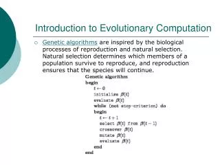
Genetic Algorithms (GA) • Population individuals are (fixed-length) binary strings (“genome”) • Start with a population of random strings. • Measure “fitness” of individuals. • Each generation forms a new population from old via recombination and mutation. • Solutions improve over generations.
Three steps to setting up a GA • 1) Devise a binary encoding representing the potential solutions to a problem. • 2) Define a fitness function. • Objective measure of quality of individual • 3) Set control parameters. • population size • maximum number of generations • probability of mutation and crossover, etc.
A1 A2 A10 A8 A6 A7 A3 A5 A9 A4 50lb 50lb 0010 1110 0001 0010 1010 1111 0001 0110 0110 1010 Example: Designing a Truss • 10 members • 16 diameters avail. • Different costs • Different strengths • Find cheapest that is strong enough • 40-bit genome • Each 4 bit sequence reps. diam. of 1 member
Running a GA • Generate an initial population of random binary strings • Calculate “fitness” of each individual • Fitness is cost of design, + penalty for fails • Create next generation • Select on the basis of “fitness” • Recombination/mating • Select some elements for mutation. • Typically one or two random bits will be flipped
00101101 00101011 10010011 10010101 Crossover in GA • Single-point crossover • There are many other forms • Randomly select crossover point • Swap crossover fragments • Offspring will have a combination of randomly selected parts of both parents Parents Children
Running a GA (continued) • Repeatedly create new generations • Calculate fitness • Terminate when an acceptable solution is been found or when the specified maximum number of generations is reached.
Running a GA/GP • Major phases of evolutionary algorithms:
Results of Truss Example • Optimal solution is known, but rare • Number of possible designs is 240 • Typical run • 200 individuals/pop.; 40 generations • Yields answer within 1% of optimal • …but examines only 8000 individuals! (.0000007% of designs)
Genetic Programming (GP) • GP is a domain-independent method for inducing programs by searching a space of S-expressions. • GP’s search technique is similar to GA’s. • The elements of a population are programs, encoded as s-expressions. • The Lisp programming language is based on s-expressions. • Original GP work was done in Lisp.
Genetic Programming Elements • S-expressions • Prefix notation • Programs, encoded as trees, evaluated via post-order traversal • Ex: tree corresponding to the S-expression • (sqrt ( / (+ a b) 2.0 ) )
Representation of a Program • S-expressions can be converted to C…. float treeFunc(float a) { if ( a > 10.0) { return 20.0; } else { return a/2.0; } } Looping constructs and subroutine calls are also possible.
Three steps to setting up a GP • Define appropriate set of functions and terminals. • Must have closure. • Functions and Terminals must be sufficient. • Define a fitness function. • Set control parameters. • GA population size, • maximum size or depth of the individual trees • size and the shape of the original trees, etc. terminal set = {a, b, c, 0, 1, 2} function set ={+, -, *, /, SQRT}
Starting a GP • Generate an initial population of random S-expression trees. • Calculate fitness value for each individual • Often over a set of test cases.
Running a GP • Create the next generation (population) • Select elements for reproduction • Random, fitness-proportionate, tournament. • Reproduce: • Direct reproduction (cloning) • Mating • Mating method differs from GA’s. • Mutation • Also differs from GA’s.
GP Crossover • Randomly choose crossover points. • Swap rooted subtrees. • “Closure” property guarantees viability of offspring
Mutation with GP • Elements that are selected for mutation will have some randomly selected node (and any subtree under it) replaced with a randomly generated subtree. • Point mutation • Tree growth (shown here)
Running a GP (continued) • Repeatedly create new generations. • Terminate when an acceptable solution is found or when a specified maximum number of generations is reached. • The termination criteria is often based on a number of hits, where a hit is defined as the successful completion of some subgoal.
Example: Santa Fe Trail • Ant animats, acquiring food. • Some gaps in trail • 89 food “pellets” • Evolve control strategy to consume all pellets • In acceptable time
Representing “Ants” T = {ahead, left, right} F ={if-food-ahead, progn2, progn3} • “Terminals” are functions, whose evaluation causes ant to move. • Fitness = # of pellets consumed in 400 terminal evaluations. • Prevents infinite runs, and weak solutions. (if-food-ahead (move) (progn2 (left) (move)))
Demo: Santa Fe Ant • During run, shows path of • best-of-generation, best-of-run • Chong, 1998
Santa Fe Ant Demo (done) • http://studentweb.cs.bham.ac.uk/~fsc/DGP.html • The applet
GP Generated Military Tactics • Squadron has a destination • Ordered either to: evade or attack • Porto, Fogel & Fogel, 1998 • Population of strategies
Generating tactics • Every 20 seconds of real time, do GP run, 40 generations. • Predicts 20 mins ahead. • Allows adaptation to changing situation. • Here, order is changed from “evade” to “attack”.
Co-evolution • Simulation uses GP-developed strategy for both squadrons.
Real-time success • Platform: Sparc 20 • Actual Pentagon military simulation. • Blue squad fires on red.
Learning to Walk with GP • Evolve control strategies for movement of arbitrarily articulated animats. • Karl Sims, 1995 • Fitness is rate of travel • physics model • LOTS of CPU cycles!
GA-learned bipedal motion • Individual strategies can be observed on theapplet. (http://www.jsh.net/andy/gat/environ.html) • User can view all trials, or just the best-of-generation. • Constrained skeletons. • Dick, 1998
Financial Symbolic Regression • The goal is time series prediction, where the target points are a financial time series. • In this case we are using a target time series derived from the daily closing prices of the S&P 500 from the years 1994 and 1995. • Uses 33 independent variables taken from time series that that are derived from the S&P 500 itself and from the closing daily prices of 32 Fidelity Select Mutual Funds. • Evett & Fernandez, 1996, 1997.
Solving Financial Problems • The top line in the graph is the daily closing price of the S&P 500. The solid line below it is the graph of the target time series after preprocessing. • The dotted line is a function evolved using GP. It is included here only as an example to illustrate that criterion for success does not require a great deal of accuracy.
The Example Evolved Function • y = (((0.38)-((-0.20923)-(FSPTX-(((-0.79706) /(0.38))*((FSUTX-FSCSX)*(FSCGX-(-0.34247))))))) *(SPX*((0.82794)/(0.54431)))) • The independent variables that were used by this evolved function are derived from the following time series. • FSPTX Fidelity select Technology Portfolio. • FSUTX Fidelity Select Utility Portfolio • FSCSX Fidelity Select Software Portfolio • FSCGX Fidelity Select Capital Goods Portfolio • SPX S&P 500 Index
Conclusions • Evolutionary algorithms are a powerful technique for problem solving in domains that: • are variable • difficult, if not impossible to optimize • GP is especially useful for problems for which the form of the solution is not known. • Evolutionary techniques are becoming widespread.
Overview of the Software • Object Oriented • C++. • Windows 95 (MS Visual C++ 5.0) • Ported to UNIX. (GNU C++) • Extended to run cooperatively on multiple machines using MPI.