Download
1 / 20
200 likes | 297 Vues
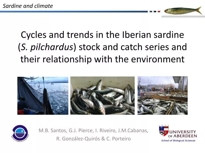
Sardine and climate. Cycles and trends in the Iberian sardine ( S. pilchardus ) stock and catch series and their relationship with the environment. M.B. Santos, G.J. Pierce, I. Riveiro , J.M. Cabanas, R. González-Quirós & C. Porteiro. VIIIb. VIIIc. BAY OF BISCAY. CANTABRIAN SEA.

E N D
Sardine and climate Cycles and trends in the Iberian sardine (S. pilchardus) stock and catch series and their relationship with the environment M.B. Santos, G.J. Pierce, I. Riveiro, J.M.Cabanas, R. González-Quirós & C. Porteiro
VIIIb VIIIc BAY OF BISCAY CANTABRIAN SEA VIIIc-West VIIIc-East IXa-North IXa-Central North IXa IXa-Central South IXa-South Portugal IXa-South Cadiz GULF OF CADIZ Sardine and climate • Single stock, delimited by Spanish-French border and Strait of Gibraltar • Supports important fishery in Spain and Portugal • Sardine has rapid growth rate, short generation time, long spawning season; females produce high number of eggs Iberian sardine
Sardine and climate • Single stock, delimited by Spanish-French border and Strait of Gibraltar • Supports important fishery in Spain and Portugal • Sardine has rapid growth rate, short generation time, long spawning season; females produce high number of eggs Iberian sardine SSB F • High importance of recruitment in overall population dynamics • Periods of consecutive low recruitments (+ high F) have led to “crises” in the fishery R
Sardine and climate Manystudieshighlightapparentenvironmentalrelationships Dickson et al, 1988 Galician upwelling v catches López-Jamar et al, 1995 Negative correlation: R v upwelling Roy et al., 1995 Wind strength v R Previous studies
Sardine and climate Stock, catch + environmental variables R, SSB series: 1978-2009 (32 y) Landings in each area 1948-2009 (62 y) Sunspots Upwelling , IPC indexes, SST, Wind, AT, CLO, etc and a series of global, regional and local environmental variables NAO, NAO winter, AMO, GULF, EA
Sardine and climate Selection of explanatory variables Exploration of collinearity in EVs + variable selection Relationships between EVs: are they correlated? Dynamic Factor Analysis (a dimension-reduction technique) to try to identify common trends in the EVs. Monthly. Best model: 1 common trend. Average value used for analysis.
Sardine and climate Modelling approach Time series = trend + cycle and/or AC + residual • Modeleach RV as function of EVs: selectbestEVs (GAM) • Quantify AC. If AC persists in modelresiduals, use GAMM • DecomposeRVs, EVsinto simple trends and residuals (GLM v time) • Compare RV trends and residualswith EV trends and residuals (whichcomponentsappeartobedrivingtherelationship?)
Sardine and climate • Exploration of time series Trends in Recruitment + SSB Possibility of linear + simple polynomial relationships with time - GLMs R SSB Linear trend in R: decreasing from high values in the 80s to low values in the 90s and now No trend in SSB
Sardine and climate Exploration of time series Cycles in Recruitment + SSB Spectral analysis (note: we are also detrending the data because we want to concentrate on the cycles) R SSB 0.25 cycle / y = 1 cycle every 4 years 0.1 cycle / y = 1 cycle every 10 years (short time series, only 32 years)
Sardine and climate • Exploration of time series (Partial) AC in Recruitment + SSB Partial autocorrelograms Recruitment: PAC significant at time lag 1 SSB: PAC very significant at time lag 1
Sardine and climate • Exploration of time series All response variables * Log transformed
Sardine and climate • Exploration of time series Explanatory variables
Sardine and climate Results:L_IXaCN GAM/GAMM : which EVs best explain Landings? Final GAM forL_IXaCN (%DE=45.6%, AIC = 20.47) • Landings are the most complex series to model as they will a priori contain stock, fishing and environment effects • AC persists in modelresiduals • GAMM with AR1 variancestructureisan “improvement” • …but AC persists and allenvironmentaleffectsthenbecome non-significant
Sardine and climate Results: SSB GAM/GAMM : which EVs best explain SSB? Final GAM for SSB (%DE=68.3%, AIC = 819.18) No autocorrelation(confirmedbycomparingAIC of bestmodelwith/withoutanAR1 variancestructure)
Sardine and climate Results: Recruitment GAM/GAMM: which EVs best explain R? Final GAM forLogR (%DE=64.6%, AIC = -17.44) No autocorrelation(confirmedbycomparingAIC of bestmodelwith/withoutanAR1 variancestructure)
Sardine and climate Results: effect of wind strength LogR v trend + noise in winter wind strength (W40350_W) GLM Extract trend and residuals (noise) from both LogR and Wind strength GAM LogRas a function of W, W trend and W noise GAM LogR noise as function of W noise Log R v W (%DE=20.2 P=0.0143) Log R v W noise (%DE=0.1 P=0.870) Log R v W trend (%DE=39.2 P=0.0001) Log R noise v W noise (%DE=0.1 P=0.837)
Sardine and climate Results: effect of SST LogR v trend + noise in winter SST (SST40350_W) GLM trend and residuals (noise) from LogR (no significant trend in SST40350_W) GAM LogR as function of SST GAM LogR trend and LogR noise as function of SST Log R v SST (%DE=35.3 P=0.0115) Log R trend v SST (%DE=13.0 P=0.289) Log R noise v SST (%DE=16.3 P=0.0219)
Sardine and climate Results: effect of sunspots LogR v trend + noise in average number of sunspots (avspots) GLM Extract trend and residuals (noise) from both LogR and Sun GAM LogRas a function of Sun, Sun trend and Sun noise GAM LogR noise as function of Sun noise LogR v Sun (%DE=25.2 P=0.0034) LogR v Sun noise (%DE=4.1 P=0.267) LogR v Sun trend (%DE=39.2 P=0.0001) LogR noise v Sun noise (%DE=8.0 P=0.116)
Sardine and climate Conclusions • In short-livedfish, environmentalrelationships can beanimportantcomponent of stock and fisherydynamics • Iberiansardine R, SSB, catch series all show “environmental” effects: • - windstrength, SST, AT, NAO, AMO, sunspots, • GAMM sometimespermitsremoval of AC (and maynotbeneeded) • Need to investigate the nature of the relationships to understand mechanisms; separating trends and noise is useful guide • Short time series remain a limitation (e.g.todetectcycles) • Relationshipsfor R: • - wind, sunspots: effectsduetoopposite/similar linear trends • - SST effect relates more to short-termvariationaroundtrend
Sardine and climate Acknowledgements WewouldliketothankallourPortuguese and Spanishcolleaguesworkingonsardine, allthecrew and scientists in theacousticsurveys, everyonewhocollectedthelandingsdata, and Alain Zuur (Highland Statistics) forstatisticaladvice Xunta de Galicia, Programa de Recursos Humanos Plan Nacional de I + D + I, Proyecto CTM 2010- 16053 (LOng-Term variability OF small-PELagic fishes at the North Iberian shelf ecosystem)