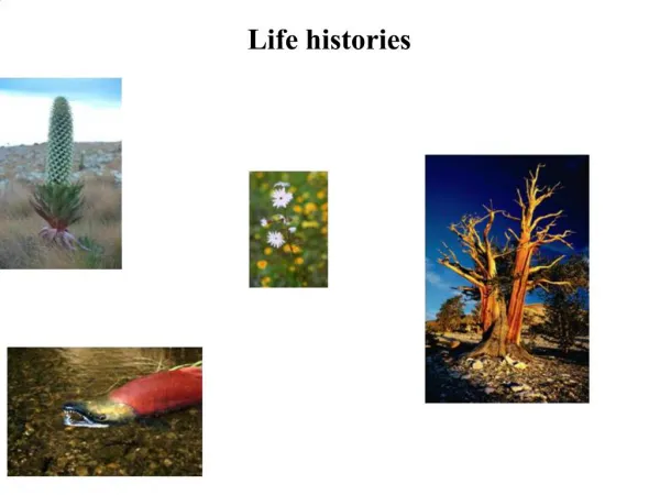
Life histories

1. Life histories

2. What is a life history? Life History – An individuals pattern of allocation, throughout life, of time and energy to various fundamental activities, such as growth, reproduction, and repair of cell and tissue damage.

3. Examples of life history traits • Size at birth • Age specific reproductive investment • Number, and size of offspring • Age at maturity • Length of life

4. Age specific reproductive investment mx Age, x

5. An extreme case: semalparity vs. iteroparity Semelparous Iteroparous Semelparity – A life history in which individuals reproduce only once in their lifetime. Iteroparity – A life history in which individuals reproduce more than once in their lifetime.

6. An example: Oncorhyncus mykiss Steelhead Rainbow trout • Live a portion of their life in saltwater • Migrate to freshwater to spawn • Often semelparous • Spend entire life in freshwater • Iteroparous

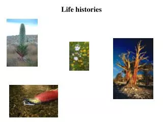
7. An example: Mt Kenya Lobelias Lobelias live on Mt Kenya from 3300-5000m!

8. Mt Kenya Lobelias Lobelia telekii (semalparous) Lobelia keniensis (iteroparous)

9. Why be semalparous vs. iteroparous? A model of annuals vs. perennials: Cole (1954) B is the # of seeds produced (assumes that all seeds survive) Based on these equations, when would the relative numbers of annuals and perennials not change?

10. Cole’s Paradox The relative abundance of annuals and perennials will not change if their per capita growth rates are equal: • An annual need only produce one more seed per generation to out-reproduce a perennial. So why are there any perennials at all?

11. A resolution to Cole’s Paradox Assumptions of Cole’s model • No adult mortality in the perennial • No juvenile mortality in either the annual or the perennial Relaxing these assumptions: Charnov and Schaffer (1973) • Adults survive each year with probability Pa • Juveniles survive to adulthood with probability Pj

12. A resolution to Cole’s Paradox

13. A resolution to Cole’s Paradox The relative abundance of annuals and perennials will not change if their per capita growth rates are equal: Which after a little algebra is: • Annuals (semalaparity) are favored by low adult survival and high juvenile survival • Perennials (iteroparity) are favored by high adult survival and low juvenile survival

14. A resolution to Cole’s Paradox BP = 1, Pj = 1/2 BP = 1, Pa = 1/2 Annuals win Annuals win BA BA Perennials win Perennials win Adult survival, Pa Juvenile survival, Pj • High rates of juvenile survival favor the evolution of annuals/semalparity • High rates of adult survival favor the evolution of perennials/iteroparity

15. A test of the theory: Mt Kenya Lobelias Lobelia keniensis (iteroparous) Lobelia telekii (semalparous) 5000m (Dry rocky slopes) 3300m (Moist valley bottoms)

16. A test of the theory: Mt Kenya Lobelias Young (1990) • Measured adult survival rates of the iteroparous species, Lobelia keniensis, at various sites along this environmental gradient • Found that adult survival decreases as elevation increases and moisture decreases • Found that the species transition zone occurs where adult survival falls below the critical threshold predicted by the model Adult mortality too high for iteroparity 5000m (Dry rocky slopes) Adult mortality sufficiently low for iteroparity 3300m (Moist valley bottoms)

17. Practice question • In order to identify the importance of density regulation in a population of wild tigers, you assembled a data set drawn from a single population for which the population size and growth rate are known over a ten year period. This data is shown below. Does this data suggest population growth in this tiger population is density dependent? Why or why not? • What problems do you see with using this data to draw conclusions about density dependence?

18. Growth rate Population size

19. Population size Year

20. Number and size of offspring All else being equal it should be best to maximize the number of offspring

21. A fundamental question Maternal resources Offspring Offspring

22. What is the best solution? The Lack Clutch – The best solution is the one that maximizes the number of offspring surviving to maturity. Lack (1947) David Lack W = S*N

23. There is a fundamental trade-off W = N*S(N) S This is the “Lack Clutch” W Number of offspring produced, N

24. An example with #’s What is the optimal number of offspring to produce in this example?

25. An example with #’s What is the optimal number of offspring to produce in this example?

26. Do real data conform to the ‘Lack Clutch’? The observed clutch sizes appear consistently smaller than the ‘Lack Clutch’ Table from Stearns, 1992

27. Where does the ‘Lack Clutch’ go wrong? Assumptions of the ‘Lack Clutch’ • No trade-off between clutch size and maternal mortality • No trade-off between clutch size across years • No parent-offspring conflict (who controls clutch size anyway?) All have been shown to be important in some real cases!

29. Life history strategies: r vs. K selection In the 1960’s interest in life histories was stimulated by the identification of two broad classes of life history STRATEGIES (MacArthur and Wilson, 1967): r selected K selected • Mature early • Have many small offspring • Make a a few large reproductive efforts • Die young • Mature later • Have few large offspring • Make many small reproductive efforts • Live a long time

30. Putative examples of r vs. K selected species Taraxacum officinale Dandelion Sequoiadendron giganteum Redwood

31. Putative examples of r vs. K selected species Peromyscus leucopus Deer mouse Gopherus agassizii Desert tortoise

32. What conditions favor r vs K species? A simple model of density-dependent natural selection can help… of this, each INDIVIDUAL contributes: to population growth

33. A simple model of density dependent selection Since an individuals contribution to population growth is intimately connected to the notion of individual fitness, we assume that the fitness of various genotypes is: Roughgarden (1971)

34. A critical assumption There is an inherent trade-off between ‘K’ and ‘r’ r K AA Aa aa Genotypes with a large ‘r’ value tend to have a small ‘K’ value

35. Can an allele that increases r but decreases K fix? N Example 1: rAA = .15 KAA = 900 rAa = .10 KAa = 950 raa = .05 Kaa = 1000 p N p N Example 2: rAA = .30 KAA = 950 rAa = .20 KAa = 975 raa = .10 Kaa = 1000 p N p Generation # In a constant environment, NO!

36. Why does the ‘r’ selected genotype lose? • In a constant environment the population will ultimately approach its carrying capacity • As the population size approaches the carrying capacity of the various genotypes, density dependent selection becomes strong • Under these conditions, genotypes with a high ‘K’are favored by natural selection

37. What about ‘disturbed’ environments? N In the examples at right, the population size is reduced (disturbed) by a random amount in each generation. p N p In this example: rAA = .30 KAA = 900 rAa = .20 KAa = 950 raa = .10 Kaa = 1000 N p p N Disturbance increases p N p N Generation #

38. Conclusions for ‘r’ and ‘K’ selection • In a constant environment the population will ultimately approach its carrying capacity and the genotype with the highest ‘K’ will become fixed • If population size remains sufficiently below the ‘K’s of the various genotypes due to random environmental disturbances or other factors, the genotype with the highest ‘r’ will become fixed in the population

39. A test of ‘r’ vs. ‘K’ selection: Dandelions and disturbance (Solbrig, 1971) • Four genotypes A-D. - Genotype ‘A’ has the largest allocation to rapid seed production - Genotype ‘D’ delays reproduction until after substantial leaf formation - Genotypes ‘B’ and ‘C’ are intermediate • Established three plots with varying levels of disturbance - Heavily disturbed by weekly lawn mowing • Moderately disturbed with monthly lawn mowing • Minimal disturbance with seasonal lawn mowing

40. Dandelions and disturbance (Solbrig, 1971) “r selected” genotype “K selected” genotype • High levels of disturbance favored the genotype with the greatest r