IB Standard level stats
420 likes | 434 Vues
Learn how to calculate mean and standard deviation, use frequency tables, and interpret data with outliers. Practice examples included.

IB Standard level stats
E N D
Presentation Transcript
IB Standard level stats Part 2
Statistics Topics left • Standard deviation – a recap • Cumulative frequency- medians, quartiles IQR, deciles, percentiles and box whisker plots • Histograms • Random variables- probability distributions, expectation • Binomial distribution • Normal distribution
Mean The mean is the most widely used average in statistics. It is found by adding up all the values in the data and dividing by how many values there are. Notation: If the data values are , then the mean is This symbol means the total of all the x values This is the mean symbol Note: The mean takes into account every piece of data, so it is affected by outliers in the data. The median is preferred over the mean if the data contains outliers or is skewed.
Mean If data are presented in a frequency table: then the mean is
Mean Example: The table shows the results of a survey into household size. Find the mean size. TOTAL 114 343 To find the mean, we add a 3rd column to the table. Mean = 343 ÷ 114 = 3.01
Standard deviation There are three commonly used measures of spread (or dispersion) – the range, the inter-quartile range and the standard deviation. The standard deviation is widely used in statistics to measure spread. It is based on all the values in the data, so it is sensitive to the presence of outliers in the data. The variance is related to the standard deviation: variance = (standard deviation)2 The following formulae can be used to find the variance and s.d.
Standard deviation Example: The mid-day temperatures (in ˚C) recorded for one week in June were: 21, 23, 24, 19, 19, 20, 21 First we find the mean: ˚C So variance = 22 ÷ 7 = 3.143 So, s.d. = 1.77 ˚C(3 s.f.) Total: 22
Standard deviation There is an alternative formula which is usually a more convenient way to find the variance: Therefore, and
Standard deviation Example (continued): Looking again at the temperature data for June: 21, 23, 24, 19, 19, 20, 21 We know that ˚C Also, = 3109 So, ˚C Note: Essentiallythe standard deviation is a measure of how close the values are to the mean value.
Calculating standard deviation from a table When the data is presented in a frequency table, the formula for finding the standard deviation needs to be adjusted slightly: Example: A class of 20 students were asked how many times they exercise in a normal week. Find the mean and the standard deviation.
Calculating standard deviation from a table TOTAL: 20 38 116 The table can be extended to help find the mean and the s.d.
Calculating standard deviation from a table If data is presented in a grouped frequency table, it is only possible to estimate the mean and the standard deviation. This is because the exact data values are not known. An estimate is obtained by using the mid-point of an interval to represent each of the values in that interval. Example: The table shows the annual mileage for the employees of an insurance company. Estimate the mean and standard deviation.
Calculating standard deviation from a table TOTAL 45 480,000 6,587,500,000 miles miles
Notes about standard deviation Here are some notes to consider about standard deviation. • In most distributions, about 67% of the data will lie within 1 standard deviation of the mean, whilst nearly all the data values will lie within 2 standard deviations of the mean. • Values that lie more than 2 standard deviations from the mean are sometimes classed as outliers – any such values should be treated carefully. • Standard deviation is measured in the same units as the original data. Variance is measured in the same units squared. • Most calculators have built-in functions which will find the standard deviation for you. Learn how to use this facility on your calculator.
Examination style question Examination style question: The ages of the people in a cinema queue one Monday afternoon are shown in the stem-and-leaf diagram: Explain why the diagram suggests that the mean and standard deviation can be sensibly used as measures of location and spread respectively. Calculate the mean and the standard deviation of the ages. The mean and the standard deviation of the ages of the people in the queue on Monday evening were 29 and 6.2 respectively. Compare the ages of the people queuing at the cinema in the afternoon with those in the evening.
Examination style question a) The mean and the standard deviation are appropriate, as the distribution of ages is roughly symmetrical and there are no outliers. b) The cinemagoers in the evening had a smaller mean age, meaning that they were, on average, younger than those in the afternoon. The standard deviation for the ages in the evening was also smaller, suggesting that the evening audience were closer together in age.
Combining sets of data Sometimes in examination questions you are asked to pool two sets of data together. Example: Six male and five female students sit an A level examination. The mean marks were 52% and 57% for the males and females respectively. The standard deviations were 14 and 18 respectively. Find the combined mean and the standard deviation for the marks of all 11 students.
Combining sets of data Let be the marks for the 6 male students. Let be the marks of the 5 female students. To find the overall mean, we first need to find the total marks for all 11 students. Therefore So the combined mean is:
Combining sets of data To find the overall standard deviation, we need to find the total of the marks squared for all 11 students. Notice that the formula rearranges to give Therefore, So the combined s.d. is: to 3 s.f.
VARIANCE - you consider how the values are spread about the mean To calculate VARIANCE, δ2, for a POPULATION For a list of data: δ2 = Σ x2 _ μ2 n For grouped data: δ2 = Σ fx2 _ μ2 Σf Remember - μ is the mean of the population As this is measured in terms of x2 then the units would be x2 - a bit strange when comparing with original values So to measure in terms of x we often calculate the STANDARD DEVIATION
STANDARD DEVIATION - the positive square root of the variance Therefore STANDARD DEVIATION, δ, of a POPULATION For a list of data: δ = Σ x2_ μ2 n For grouped data: δ = Σ fx2 _ μ2 Σf √ √
This is the whole POPULATION For a list of data: δ2 = Σ x2 _ μ2 n Σ x2 = Σ x = n = So μ = Σ x n δ2 =
∑ fx = 1340 ∑ f = 150 So μ = 8.93 ∑ fx2 = 17560 δ2 = Σ fx2 _ μ2 Σf δ2 = 17560 _ 8.93 2 150 = 37.32 δ = 6.11
Quartiles and box plots A set of data can be summarised using 5 key statistics: • the median value (denoted Q2) – this is the middle number once the data has been written in order. If there are n numbers in order, the median lies in position ½ (n + 1). • the lower quartile (Q1) – this value lies one quarter of the way through the ordered data; • the upper quartile (Q3) – this lies three quarters of the way through the distribution. • the smallest value • and the largest value.
Note: The box width is the inter-quartile range. Inter-quartile range = Q3 – Q1 Quartiles and box plots These five numbers can be shown on a simple diagram known as a box-and-whisker plot (or box plot): Smallest value Q1 Q2 Q3 Largest value The inter-quartile range is a measure of spread. The semi-inter-quartile range = ½ (Q3 – Q1).
Quartiles and box plots Example: The (ordered) ages of 15 brides marrying at a registry office one month in 1991 were: 18, 20, 20, 22, 23, 23, 25, 26, 29, 30, 32, 34, 38, 44, 53 The median is the ½(15 + 1) = 8th number. So,Q2 = 26. The lower quartile is the median of the numbers below Q2, So, Q1 = 22 The upper quartile is the median of the numbers above Q2, So, Q3 = 34. The smallest and largest numbers are 18 and 53.
Quartiles and box plots The (ordered) ages of 12 brides marrying at the registry office in the same month in 2005 were: 21, 24, 25, 25, 27, 28, 31, 34, 37, 43, 47, 61 Q2 is half-way between the 6th and 7th numbers: Q2 = 29.5. Q1 is the median of the smallest 6 numbers: Q1 = 25 Q3 is the median of the highest 6 numbers: Q3 = 40. The smallest and highest numbers are 21 and 61.
Quartiles and box plots A box plot to compare the ages of brides in 1991 and 2005 It is important that the two box plots are drawn on the same scale. We can use the box plots to compare the two distributions. The median values show that the brides in 1991 were generally younger than in 2005. The inter-quartile range was larger in 2005 meaning that that there was greater variation in the ages of brides in 2005. Note: When asked to compare data, always write your comparisons in the context of the question.
Cumulative frequency diagrams A cumulative frequency diagram is useful for finding the median and the quartiles from data given in a grouped frequency table. There are some important points to remember: • the cumulative frequencies should be plotted above the upper class boundaries of the intervals – don’t use the mid-point. • points can be joined by a straight line (for a cumulative frequency polygon) or by a curve (for a cumulative frequency curve). A cumulative frequency polygon
Cumulative frequency diagrams Example: A survey was carried out into the number of hours a group of employees worked. The upper class boundary (u.c.b.) of the first interval is actually 9.5 (as it contains all values from 0.5 up to 9.5). The table below shows the cumulative frequencies:
You don’t need to add 1 before halving the frequency when the data is cumulative Cumulative frequency diagrams As well as plotting the points given in the previous table, we also plot the point (0.5, 0) – no one worked less than 0.5 hours. We can estimate the median by drawing a line across at one half of the total frequency, i.e. at 70. We see that Q2 ≈ 43. For the lower quartile, a line is drawn at 0.25 × 140 = 35. This gives Q1 ≈ 36. Drawing a line at 0.75 × 140 = 105, we see that Q3 ≈ 48. So the inter-quartile range is 48 – 36 = 12.
Cumulative frequency diagrams Percentiles and deciles Instead of looking at quartiles we can also split the data up in terms of tenths (deciles) and hundredths (percentiles) We can estimate the 3rd decile by drawing a line across at 3/10 of the total frequency, i.e. at 42. We see that D3 ≈ . For the 7th decile, a line is drawn at 0.7 × 140 = 98. This gives D7 ≈ . .
Cumulative frequency diagrams Examination style question: The cumulative frequency diagram shows the marks achieved by 220 students in a maths examination. a) Estimate the median and the 95th percentile. b) Where should the pass mark of the examination be set if the college wishes 70% of candidates to pass?
Cumulative frequency diagrams a) The median will be approximately the 220 ÷ 2 = 110th value. This is about 61%. The 95th percentile lies 95% of the way through the data. A line is drawn across at 0.95 × 220 = 209.This gives a mark of 84%.
Cumulative frequency diagrams • The college wants 70% of 220 = 154 students to pass. Therefore 66 students will get a mark below the pass mark. • Drawing a line across at 66 gives a pass mark of about 55%.
Histograms A histogram can be used to display grouped continuous data. There are some important points to remember: • The area of each bar in a histogram should be in proportion to the frequency. • When the class widths are not all equal, proportional areas can be achieved by plotting the frequency density on the vertical axis, where • The class width of an interval is calculated as the difference between the smallest and largest values that could occur in that interval. Upper class boundary minus lower class boundary
Notice that the class widths are not all equal – frequency densities need to be used. Histograms Example: 50 overweight adults tested a new diet. The table shows the amount of weight they lost (in kg) in 6 months.
Histograms Histogram to show weight loss When you draw a histogram, remember to: • plot the frequency densities on the vertical axis; • choose sensible scales for your axes; • label both your axes; • give the histogram a title.
Histograms Histogram to show weight loss We can use the histogram to estimate, for example, the number of people who lost at least 12kg: • There were 2 people who lost between 15 and 25 kg. • To estimate how many people lost between 12 and 15 kg, times this new class width by the frequency density for that class: 3 × 1 = 3. • That means that about 5 people lost at least 12 kg.
The measurements are to the nearest millimetre. The first interval actually contains all wing spans between 194.5 and 204.5 mm The measurements are to the nearest millimetre. The first interval contains all wing spans between 194.5 and 204.5 mm Histograms Example: An ornithologist measures the wing spans (to the nearest mm) of 40 adult robins. Her results are shown below. The last interval is open-ended. We assume that its width is twice that of the previous interval.
Histograms Example (continued) A histogram showing the wing spans of robins Freq. density Wing span (mm)