Download
1 / 26
260 likes | 279 Vues
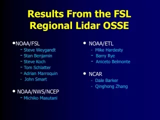
NOAA/FSL Steve Weygandt Stan Benjamin Steve Koch Tom Schlatter Adrian Marroquin - John Smart NOAA/NWS/NCEP Michiko Masutani. Results From the FSL Regional Lidar OSSE. NOAA/ETL - Mike Hardesty Barry Rye Aniceto Belmonte NCAR - Dale Barker - Qinghong Zhang.

E N D
NOAA/FSL • Steve Weygandt • Stan Benjamin • Steve Koch • Tom Schlatter • Adrian Marroquin • - John Smart • NOAA/NWS/NCEP • Michiko Masutani Results From the FSL Regional Lidar OSSE • NOAA/ETL • - Mike Hardesty • Barry Rye • Aniceto Belmonte • NCAR • - Dale Barker • - Qinghong Zhang
Assess forecast impact of wind observations • from a Doppler lidar flown aboard a polar orbiting satellite • Evaluate efficacy of different lidar scan • strategies • Refine processing/assimilationtechniques • for space-based Doppler lidar wind obs Goals of lidar Observing System Simulation Experiments
Regional models behave very differently than global models • Typically run overdata-rich regions • Utilize high-frequency assimilation • Better resolve local forcing from surface features • Influenced byobs assimilation andboundary conditions • Potential impact of lidar obs for mesoscale systems not well unknown • Spatial variability of mesoscale impact over CONUS not well known Motivation for Regional OSSE
Nature Run OSSE Experiment Global Boundary Conditions ECMWF Global Nature Run MM5 Regional Nature Run Gridded output Gridded output Simulated Observations Simulated Observations Global Verification Regional Verification Gridded output Gridded output RUC Regional OSSE Experiment MRF Global OSSE Experiment Boundary Conditions Regional Relationship between Global and Regional OSSEs
MM5 REGIONAL NATURE RUN • Model Physics • Kain-Fritsch cu. param., Schultz microphysics • Burk-Thompson PBL, RUC Land Surface Model • RRTM radiation formulation • Model Grid • 10-km horizontal grid spacing (740 x 520) • 43 sigma levels (top = 20 km, const. spacing ~800 m) • Model Data • Initial, boundary data from ECMWF nature run
RUC REGIONAL ASSIMILATION RUN • Model Physics • Grell ensemble cu. param., Reisner microphysics • Burk-Thompson PBL, RUC Land Surface Model • Dudhia radiation formulation • Model Grid • 40-km horizontal grid spacing (151 x 113) • 50 hybrid levels (top = 450 K, variable spacing) • Model Data • Initial, boundary data from MRF global experiments • Simulated observations from MM5 nature run
15 16 17 18 19 20 21 Verification RUC MM5 EC Feb 11 12 13 14 15 16 17 18 19 20 21 22 Regional Assimilation Configuration • RUC 3DVAR (Zunb,u, v, qv, lnQ) • 3-h update cycle (previous RUC fcst) • 6-h BC updates (matched MRF expt.) • Start RUC 00z 13 Feb (MRF 1st guess) • 48-h fcst (00z,12z); 18-h fcst (06z,18z) • Grid verification to MM5 (15 Feb – 20 Feb)
LIDAR FORWARD MODEL GEOMETRY (schematic only, actual model includes earth curvature) Lidar LOS wind components: RUC analyzes horizontal wind: Assume vertical velocity small compared to horizontal velocity:
Lidar Simulation Details • Direct detection (molecular) Doppler lidar • Low satellite orbit (450 km) • 20-W trans., 355 nm, 1-m telescope, 5-sec avg. • Cloud effects from model ice and liquid water • water clouds opaque • ice clouds use backscatter, extinction from model ice water • “ideal” lidar for initial study (match global strategy) • 8 “stares” per sec, 5 shots per stare (over 35 km) • Dual-look scanning of the same region
8-POINT SCAN Nadir Angle: 45° Azimuth Angles: 36.65°, 136.07°, 19.18°, 153.53°, -26.47°, -160.82°, -43.94°, -143.36° 0 1 2 3 -1 11 4 9 Forward 5 -2 12 3 10 6 1 7 4 15 2 8 13 -3 9 Latitude [degrees] 7 16 10 14 5 -4 11 6 8 12 Aft 13 -5 14 15 -6 16 -4 -3 -2 -1 0 1 2 3 Longitude [degrees]
Forward Forward Forward Aft Aft Aft 8-POINT SCAN Nadir Angle: 45° Shot Pattern 0 -2 -4 -6 -8 -10 Latitude [degrees] -12 -14 -16 -18 -20 -4 -3 -2 -1 0 1 2 3 Longitude [degrees]
110 | 120 | 100 | 80 | 60 | 130 | 90 | 70 | LOCATION OF NS LIDAR PASSES Longitude 0000z 0435z 0304z 0132z
Observation Error Standard Deviations Observation Type Error Std. Dev Rawinsonde H 6.5 - 26.0 m Rawinsonde T 0.4 K Rawinsonde ln Qv 0.1 - 0.2 Rawinsonde U,V 0.8 - 1.4 m/s ACARS T 1.0 K ACARS U,V 1.5 m/s Profiler U,V 1.0 m/s VAD U,V 1.0 m/s Surface U,V 0.5 m/s Lidar Vr 1.0 m/s
OSSE OB DATA COUNTS Approximate no. of obs data points Ob typeVariables12z15z Raob (Z,T,Q,U,V) 3700 0 Prof/VAD (U,V) 2600 2600 ACARS (T,U,V) 1200 1300 METAR/Buoy(T,Q,U,V) 1600 1600 Lidar (Vr) 1500 1500 • Lidar adds ~8% more wind obs at • raob init times (00z, 12z) • Lidar adds ~14% more wind obs at • non raob init times (06z, 18z)
LIDAR EXPERIMENTS MRF Expt. Boundary Observations NameConditions Assimilated StdNonestandard obsnone StdStdstandard obsstandard StdNoAcstandard obsstandard - aircraft StdLid standard obsstandard + ideal lidar LidNonestandard + lidar obsnone LidStdstandard + lidar obs standard LidLid standard + lidar obs standard + ideal lidar LidLidrstandard + lidar obs standard + realistic lidar x x x x x (CNTL)
No obs (BC only) Non-raob init time (06z,18z) Std obs Raob init time (00z,12z) • Realistic error growth with standard obs assimilation • Errors slightly larger for non-raob initialization times
How well does the simulated data impact • (OSSE) match real data impact (OSE) ? • Compare ACARS obs denial for: • Real data OSE: 4-16 Feb 2001 • Simulated data OSSE: 15-20 Feb 1993 • Many differences between OSSE and OSE • Different weather • Different observation errors • Different number ACARS obs • Different verification (raob vs. grid) Regional OSSE Calibration
Denying ACARS degrades both OSSE & OSE fcsts • Greatest impact at upper-levels for both OSSE, OSE 4-16 Feb 2001 15-20 Feb 1993 06z, 18z init 06z, 18z init StdStd StdNoAc Real Data Simulated Data Verified against MM5 nature run (no errors) Verified against raobs with unknown errors
Normalize Errors “% Improvement”=- (% change error)= CNTLerror – EXPerrorCNTLerror POS = fcst better NEG = fcst worse • Fcst degradation from denying • ACARS similar for OSE, OSSE
Lidar obs assimilation reduces forecast error • Error reduction greater for non-raob init times • Error reduction decreases with forecast length Non-raob init time (06z,18z) Raob init time (00z,12z) Std obs Std obs+lidar Err sd=1 m/s
~5% improvement in 6-h forecast from lidar obs • Additional improvement likely from use of • boundary conditions which contain lidar obs Std obs+lidar Err sd=1 m/s Non-raob init time (06z,18z) Raob init time (00z,12z)
Lidar obs reduce forecast error at all levels • Reduction greater for non-raob init times Raob init time (00z,12z) Non-raob init time (06z,18z)
Lidar obs improve fcst more at non-raob init times • Lidar obs improvement greatest aloft
Forecast error characteristics for regional assimilation system appear realistic • ACARS denial comparison against real-data OSE yields good agreement • Regional assimilation of lidar obs produces modest short-term wind fcst improvement • Lidar obs-related fcst improvement slight for other variables Results Summary
Observation impact strongly dependent on observation error specification • Representative errors • Systematic errors • Need realistic model depiction of clouds for realistic lidar obs simulation • Drift of regional NR from global NR complicates interpretation of BC impacts Regional OSSE Issues
Regional expts. using MRF boundary conditions containing lidar obs • Relative forecast improvement from BCs vs. assimilation • Effect of BCs on regional assimilation impact • Regional expts. using more realistic lidar obs • Evaluate lidar ob impact for specific cases • Examine spatial variability of lidar ob impact Ongoing Work