The Goods Market
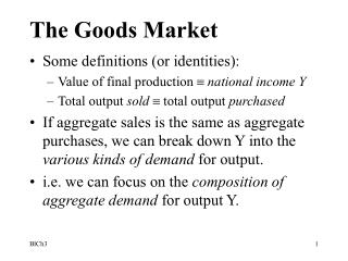
The Goods Market. Some definitions (or identities): Value of final production national income Y Total output sold total output purchased If aggregate sales is the same as aggregate purchases, we can break down Y into the various kinds of demand for output.

The Goods Market
E N D
Presentation Transcript
The Goods Market • Some definitions (or identities): • Value of final production national income Y • Total output sold total output purchased • If aggregate sales is the same as aggregate purchases, we can break down Y into the various kinds of demand for output. • i.e. we can focus on the compositionof aggregate demand for output Y.
Composition of aggregate demand Z • Consumption C • Investment I • Fixed • Residential (consumers) • Non residential (firms) • Inventories • Government spending G • Net exports NX • Exports X • Less Imports IM
Consumption • Goods and services purchased by consumers • Some might be some sort of investment like durables • Investment (not financial) • Firms invest in new plants and equipments • Consumers invest in new houses • Government spending (on goods and services only) • Excludes transfers (e.g. medicare, S.S.) • and interest payments on gov’t debt • (total would be called government expenditures)
Exports are foreign demand for domestic goods and services (demand for Y) so they should be included as demand for domestic output. • Imports are domestic demand for foreign goods (goods produced abroad) - they should not be included in Y as they are not demand for domestic output. However as they are already included in consumption and other purchases they must be subtracted. • Net Exports = Exports - Imports
Inventories corresponds to goods that were produced during a certain year I.e. during a specific accounting period but were not sold during the same accounting period. • To get an accurate account of production during the year, we must • Subtract inventories at the beginning of the year (they were produced in the previous year) • Add inventories at the end of the year (produced this year but not sold)
Determination of aggregate demand Z • By definition (identity): Z C + I + G + X - IM in an open economy Z C + I + G in a closed economy • Let’s assume • Fixed prices (short run Keynesian model) • One good (everything is in real term) • Closed economy
Short run - medium run - long run • Short run - period too short to allow prices to adjust - fixed prices - unemployment possible • Medium run - economy is always at full employment (labor market must adjust) - prices adjust to bring economy back to full employment - capital stock is fixed • Long run - growth theory - capital stock increases through investment in the economy
Determinants of consumption C • Let’s define YD - disposable income - as YD Y - Tax + Transfer or Y - T (T is net tax) • Consumption is determined by disposable income: C increases as YD increases • so consumption is a positive function of YD C = C(YD) = C(Y-T) this is a behavioral relation which can be specified with the following linear form: C = co + c1 YD c1 is the MPC
Consumption function C C = C(YD) Slope = c1 co YD=Y-T
Endogenous versus exogenous variables • Definition • Endogenous variables are determined within the model e.g. C , Y and YD • Exogenous variables are determined outside of the model, i.e. they are independent of any other variable in the model • Investment I is considered as an exogenous variable in this chapter • Government spending G and taxes T are also exogenous variables - they are policy instruments for the government.
Model • C = c0 + c1 (Y-T) • I = I (exogenous - given) • G = G (exogenous - policy variable) • Z C + I + G by definition • Y = Z (equilibrium condition)
Algebraic Solution • Since in equilibrium, supply of goods (Y) should be equal to aggregate demand (Z), by replacing we get: • Y = c0 + c1 (Y-T) + I + G = c0 + c1Y -c1T + I + G 1/(1-c1) is the multiplier m and (c0 + I + G - c1T) is autonomous spending Z0
Graphical solution Y=Z Z Z = Z0+c1Y Slope = 1 Slope = c1 Z0 Y Ye
The multiplier • Assume a specific consumption function C = 500 + .8(Y-T) i.e. MPC = .8 The multiplier m = 1/(1-c1) = 5 Since Ye = m (c0 + I + G - c1T) If G increases by ∆G, Y will increase by ∆Y = m ∆G In the example above an increase in G equal to 100 will result in an increase in Y of 500
Effect of an increase in G Z Y=Z Z’ = Z0+ ∆G +c1Y Z = Z0+c1Y 4 2 3 1 ∆G Z0 Y Ye Y’e ∆Y
Explanation • Starting at 1, the economy is in equilibrium. • An increase in G equal to ∆G immediately translates into an equal increase in aggregate demand : 1 to 2 • In 2 the economy is not in equilibrium as Z > Y so firms must increase production by ∆G to meet the additional demand: from 2 to 3 • In 3 the economy is still not in equilibrium (below ZZ’) • As production increases by ∆G , income increases equally so consumption demand will increase by c1 ∆G: this is an additional increase in aggregate demand : 3 to 4 • Then production must increase again by c1 ∆G this time to meet this new increase in aggregate demand and so on…
Rational • Production (income) depends on demand as Y = Z in equilibrium • Demand depends on income as Z = C + I + G andC = C(Y)
When there is an exogenous increase in demand, production will increase equally, and this increase in production (i.e. in income) results in an additional increase in demand. • However the additional increase in demand is smaller than the original increase because the marginal propensity to consume is less than 1 (some of the increase in income is saved): this process will not result in an infinite increase in output as the additional increases in demand get smaller and smaller and tend towards zero.
Alternative approach: Investment = saving • Approach used by Keynes in the “General Theory of Employment, Interest and Money” 1936 • By definition, private saving is what is not consumed out of disposable income: Sp YD - C hence Sp Y - T - C or Y C + Sp + T • The equilibrium condition of the model above was: Y = C + I + G By replacing, it becomes I = Sp + T - G
Interpretation • In a one person economy, investment equals savings because the decision to save and to invest is made by the same person. e.g. Robinson Crusoe’s island
Role of government: • In the above equation, the government • takes a share of income in the form of tax • spends it in the economy in the form of G so T - G corresponds to the amount of tax receipts that the government did not spend, i.e. that the government saved. • In sum, T - G (the budget surplus) can be interpreted as the government saving Sg.
Solution of the model using the alternative equilibrium condition • Let’s derive the saving function from the consumption function (c1 is the MPC) • C = c0 + c1YD and Sp YD - C • SP = YD - c0 - c1YD = - c0 + (1 - c1)YD • Sp = - c0 + (1 - c1)(Y - T) with MPS = (1 - c1) • Note that MPC + MPS = 1 as mentioned earlier • We can now use the saving function and the new equilibrium condition to find equilibrium Y (Ye)
I = Sp + (T - G) (equilibrium condition) = - c0 + (1 - c1)(Y - T) + T - G = - c0 + (1 - c1)Y - (1 - c1)T + T - G = - c0 + (1 - c1)Y - T + c1T + T - G (1 - c1)Y = c0 + I + G - c1T Finally as before.
Problem # 2 P. 62 C = 160 + 0.6 YD I = 150 G = 150 T = 100 a. In equilibrium Y = 160 + 0.6 (Y-T) + 150 + 150 i.e. Y - 0.6Y = 160 - (0.6*T) + 150 + 150 Y = [1/(1-0.6)] (160 - 60 + 150 + 150) Y = 2.5 * 400 = 1000
b. YD = Y - T = 1000 - 100 = 900 • C = 160 + 0.6*900 = 700 Problem # 3 a. Z = C + I + G = 700 + 150 + 150 = 1000 so Y = Z = 1000 (equilibrium condition) • If G = 110 ∆G = - 40 as the multiplier m = 2.5 and ∆Y = m ∆G ∆Y = - 100 and the new equilibrium Y is 900 consumption drops by c1* ∆Y or - 60 to 640 And Z = C’ + I + G’ = 640 + 150 + 110 = 900
Private savings Sp = Y - T - C = 900 - 100 - 640 = 160 Government savings Sg = T - G = 100 - 110 = -10 Equilibrium condition: I = Sp + Sg 150 = 160 - 10 = 150