Quantitative Summarization in Biostatistics Practice
350 likes | 437 Vues
Learn about summarizing experiment results, confidence intervals, and prediction intervals in biostatistics. Understand the importance of measuring and analyzing data independently for valid statistical analyses. Explore descriptive statistics and graphical aids for effective data interpretation.

Quantitative Summarization in Biostatistics Practice
E N D
Presentation Transcript
Biostatistics in Practice Session 2: Summarization of Quantitative Information Youngju Pak Biostatistician http://research.LABioMed.org/Biostat
Topics for this Session Experimental Units Independence of Measurements Graphs: Summarizing Results Graphs: Aids for Analysis Summary Measures Confidence Intervals Prediction Intervals
Units and Independence Experiments may be designed such that each measurement does not give additional independent information. Many basic statistical methods require that measurements are “independent” for the analysis to be valid. In mathematics, two events are independent if and only if the occurrence of one event makes it neither more nor less probable that the other occurs.
Population parameter Population Confidence Interval for population parameter Sampling mechanism: random sample or convenience sample Sample Sample estimate of population parameter
Experimental Units in Case Study What is the experimental unit in this study? 1. School 2. Child 3. Parent 4. GHA score (results from three diets) Are all GHA scores(eg. 153 x 3 groups=459 GHA scores for 3-4 years old children) The analysis MUST incorporate this possible correlation (clustering) if there exists.
Common Descriptive Statistics used Sample Mean and Standard Deviation (SD)Sample Median and Inter-Quartile Range (IRQ)Sample CorrelationSample Survival ProbabilitySample Risks & Odds
Mean What most people think of as “average” Easy to calculate Easily distorted Be cautious with SKEWED data Calculate: sum of data / number of data points Median Relatively easy to obtain Not affected by extreme values so it is considered a “ROBUST” statistic Calculate: Sort data If odd number points, the middle is the median Otherwise, the median is the average of the middle two numbers Mean vs. Median(measure the central tendency)
Standard Deviation (SD) &Inter-Quartile Range(IRQ)(measuring the variability or scatterness of the data ) • Inter-Quartile Range (IQR)= 75th percentile (Q3) - 25th percentile(Q1) , where 25% of the data <Q1 , 75% of the data < Q3 • SD is usually used for the normally distributed data (bellshape, symmetric around the mean) • IQR is usually used when the data distribution is skewed. • Range = Max -Min
Summarization of the Case Study How are the outcome measures summarized? e.g., Table 2:
Summary Statistics:Relative Likelihood of an Event Compare groups A and B on mortality. Relative Risk = ProbA[Death] / ProbB[Death] where Prob[Death] ≈ Deaths per 100 Persons Odds Ratio = OddsA[Death] / OddsB[Death] where Odds= Prob[Death] / Prob[Survival] Hazard Ratio≈ IA[Death] / IB[Death] where I = Incidence = Deaths per 100 PersonDays
Data Graphical DisplaysMany of the following examples are from StatisticalPractice.com Histogram Scatter plot Raw Data Summarized* * Raw data version is a stem-leaf plot. We will see one later.
Data Graphical Displays Dot Plot Box Plot Raw Data Summarized
Data Graphical Displays Line or Profile Plot Summarized - bars can represent various types of ranges
Data Graphical Displays Kaplan-Meier Plot (Source: www.cancerguide.org)
Graphical Aids for Analysis Most statistical analyses involve modeling. Parametric methods (t-test, ANOVA, Χ2) have stronger requirements than non-parametric methods (rank -based). Every method is based on data satisfying certain requirements. Many of these requirements can be assessed with some useful common graphics.
Look at the Data for Analysis Requirements • What do we look for? • In Histograms (one variable): • Ideal: Symmetric, bell-shaped. • Potential Problems: • Skewness. • Multiple peaks. • Many values at, say, 0, and bell-shaped otherwise. • Outliers.
Example Histogram: OK for Typical* Analyses • Symmetric. • One peak. • Roughly bell-shaped. • No outliers. *Typical: mean, SD, confidence intervals, to be discussed in later slides.
Z- Score = (Measure - Mean)/SD Mean = 60.6 min.SD = 9.6 min. Standardizes a measure to have mean=0 and SD=1. Z-scores make different measures comparable. 41 61 79 Mean = 0SD = 1 Mean = 60.6 min. SD = 9.6 min. -2 0 2 Z-Score = (Time-60.6)/9.6
Outcome Measure in Case Study GHA = Global Hyperactivity Aggregate For each child at each time: Z1 = Z-Score for ADHD from Teachers Z2 = Z-Score for WWP from Parents Z3 = Z-Score for ADHD in Classroom Z4 = Z-Score for Conner on Computer , where weekly score=changes from T0 All have higher values ↔ more hyperactive. Z’s make each measure scaled similarly. GHA= Mean of Z1, Z2, Z3, Z4
Summary Statistics:Rule of Thumb • For bell-shaped distributions of data (“normally” distributed): • ~ 68% of values are within mean ±1 SD • ~ 95% of values are within mean ±2 SD • “(Normal) Reference Range” • ~ 99.7% of values are within mean ±3 SD
Histograms: Not OK for Typical Analyses Skewed Multi-Peak Need to transform intensity to another scale, e.g. Log(intensity) Need to summarize with percentiles, not mean.
Look at the Data for Analysis Requirements • What do we look for? • In Scatter Plots (two variables): • Ideal: Football-shaped; ellipse. • Potential Problems: • Outliers. • Funnel-shaped. • Gap with no values for one or both variables.
Summary Statistics:Two Variables (Correlation) • Always look at scatterplot. • Correlation, r, ranges from -1 (perfect inverse relation) to +1 (perfect direct). Zero=no relation. • Specific to the ranges of the two variables. • Typically, cannot extrapolate to populations with other ranges. • Measures association, not causation. • We will examine details in Session 5.
Correlation Depends on Range of Data A B Graph B contains only the points from graph A that are in the ellipse. Correlation is reduced in graph B. Thus: correlation between two quantities may be quite different in different study populations.
Correlation and Measurement Precision A B overall 12 10 r=0 for s 5 6 B A lack of correlation for the subpopulation with 5<x<6 may be due to inability to measure x and y well. Lack of evidence of association is not evidence of lack of association.
Confidence Interval (CI) • How well your sample mean(m) reflects the true( or population) mean How confident? 95%? • A confidence interval (CI) is one of inferential statistics that estimate the true unknown parameter using interval scales.
Confidence Interval for Population Mean 95% Reference range or “Normal Range”, is sample mean ± 2(SD) _____________________________________ 95% Confidence interval (CI) for the (true, but unknown) mean for the entire population is sample mean ± 2(SD/√N) SD/√N is called “Std Error of the Mean” (SEM)
Confidence Interval: Case Study Table 2 Adjusted CI 0.13 -0.12 -0.37 Confidence Interval: -0.14 ±1.99(1.04/√73) = -0.14 ± 0.24 → -0.38 to 0.10 close to Normal Range: -0.14 ±1.99(1.04) = -0.14 ± 2.07 → -2.21 to 1.93