Download
1 / 46
460 likes | 693 Vues
Chaotic Dynamics of Near Earth Asteroids. Chaos. Sensitivity of orbital evolution to a tiny change of the initial orbit is the defining property of chaos – your integrations show that the dynamics of Near Earth Asteroids (NEAs) is chaotic!

E N D
Chaos Sensitivity of orbital evolution to a tiny change of the initial orbit is the defining property of chaos – your integrations show that the dynamics of Near Earth Asteroids (NEAs) is chaotic! This property is fundamental: the initial orbit is never known exactly (observation errors, limitations of the orbit determination algorithm, what else?) Note that chaos does not appear because the dynamics of point masses include some random element. To the contrary, the Newtonian equations describing their motion are deterministic (i.e., each orbit follows a well defined and unique trajectory)
How to quantify chaos? The Lyapunov exponent characterizes the rate of exponential divergence of nearby orbits It is formally defined as: Therefore, if d(t) = d0 exp n(t-t0), then λ = n, andλ = 0otherwise The rate of divergence may depend on the orientation of the d0 vector nearby trajectory d(t) d0 trajectory
Lyapunov Exponent The Lyapunov exponent can be computed numerically by following nearby trajectories with SwIFT, but problems may occur since d(t) must be infinitesimally small. (These problems can be avoided by using renormalization or variational equations.) Also, for a random choice of the initial orientation of the d0 vector, the computed λ corresponds to the direction of the largest stretching rate, and is therefore called the Maximum Lyapunov Exponent or MLE. The inverse of the MLE, Lyapunov time TLyap, tells us the time scale on which the orbits become unpredictable. For example, if the initial precision of orbits is 10-4, macroscopic changes of order of unity will occur due to chaos on ~10 TLyap since 10-4e10 > 1. Even if your orbit were accurate at the (absurd) level of 10-46, you couldn’t predict where the body would be after 106 TLyap.
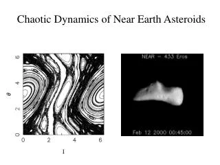
How can we study chaos? There are several additional methods that can describe different aspectsof chaos, such as the Surface of Section, Frequency Analysis, etc. To illustrate these methods, we use the fact that complex dynamical systems (such as, e.g., NEA dynamics) can often be reduced to an algebraic mapping that captures the behavior of the main variables Specifically, a 1-dimensional mapping can be constructed for any 2-dimensional Hamiltonian system by following intersections of a trajectory with some surface (called a Surface of Section or SOS) For example, near-resonant asteroidal dynamics can be reduced tothe so-called Standard Map that describes behavior of action I (semi-major axis or eccentricity) and angle θ(proxy for resonant angle)
Standard Map – fast and easy to program! “Kicked Rotor” ↑ Kick parameter http://www.scholarpedia.org/article/Chirikov_standard_map
Trojans of Jupiter (and Neptune) librate around L4 and L5. Resonant angle = λ - λJ
Surfaces of Section for the Standard Map ε = 0 (regular motion) ε = 9 (strong chaos)
No perturbation (ε = 0) Action stays constant. Angle changes at a constant rate. Like the two-body problem. Planet goes around Sun forever in the same orbit.
ε = 0 ε = 9
Weak perturbation One or two dominant frequencies of variation
Θ I
Frequency Analysis The Surface of Section (SOS) is useful because it can easily reveal the global behavior of a dynamical system and its dependence on parameters The disadvantage is that it can be difficult to reduce a complexdynamical system (e.g., NEA dynamics) to 2 degrees of freedom Frequency Analysis is also a global method but, unlike SOS, allows us to study chaos in complex systems directly by using N-body simulations For convenience, we will illustrate Frequency Analysis on the Standard Map. Examples of its application to asteroid (& Kuiper Belt) dynamics can be found in Robutel & Laskar (2001, Icarus 152, 4-28)
Real solar system Slightly different solar system
Frequency Analysis of the Standard Map Red = fast diffusion ε = 1 0 2 4 6 0 2 4 6
Frequency Analysis of the Solar System Eccentricity Semi-major Axis (AU)
Dynamics of Near Earth Asteroids NEA orbits are typically strongly chaotic, with the Lyapunov time, the inverse of the maximum Lyapunov exponent, being only ~ 100 years! Chaos appears due to a combination of frequent encounters of NEAs with the terrestrial planets and various orbital resonances As chaos typically causes gross changes in orbits in ~10TLyap, the evolution of individual NEAs is unpredictable on time scales >1000 years (annoying but still better than a weather forecast) So what’s the point of following trajectories for > 1000 years???
Lyapunov Times of Near-Earth Asteroids Lyapunov times are ~ the interval between “close” approaches to planets. Stadium billiards Tancredi (1999)
Dynamics of Near Earth Asteroids What’s the point of following trajectories over > 1000 years??? The point is that the future evolution can be predicted statistically, i.e., by identifying all possible trajectories and finding their probabilities of occurrence To obtain such a statistical description, you used an N-body integrator and, in addition to the nominal orbit, you also followed clones that started from slightly different orbits All these trajectories are correct and equally probable. You may not have had enough time to obtain full statistical description. Projects may take many months of CPU time to complete.
Example for asteroid Itokawa Hayabusa spacecraft at Itokawa Itokawa’s long axis is 535 meters long Hayabusa back to Earth (with sample?)
a = 1.324 AU, e = 0.280, i = 1.622o Discovered 1998 http://commons.wikimedia.org/wiki/File:Itokawa-orbit.svg
Example for asteroid Itokawa Individual clones Residence time distributions Itokawa may impact the Earth in the distant future, but we can’t say for sure. Michel & Yoshikawa 2005 This specific clone collides with the Earth at 3.5 My
Dynamics of Near Earth Asteroids Orbits of NEAs are short-lived. Mean dynamical lifetime is ~4 My, i.e., ~1000x shorter than the age of the solar system! Why they are not long gone??? Observed NEAs must have been inserted into their present orbits only a few My ago. How? From where? What would happen if, instead of following the orbits into the future, we would follow them into the past??? Could such integrations be used to determine where NEAs come from? Unfortunately not! On timescales exceeding TLyap, chaotic orbits tend to explore all available space in much the same way molecules would expand into empty space from a leaking oxygen tank
Dynamics of Near Earth Asteroids Backward integration over times significantly exceeding TLyap is in fact equivalent to the forward integration over the same time interval So, how can we learn anything about the origin of NEAs??? First we need to identify potential sources… can you guess?
Main Asteroid Belt: ~1 million bodies with diameters >1 km between orbits of Mars and Jupiter
Main Asteroid Belt as a source of NEAs: objects slowlyleak out of the main belt via resonances such as υ6 or 3:1
Residence Time Distribution • Results for υ6 resonance • Distribution shows where NEAs are statistically likely to spend their time • 70% of NEAs from the υ6 resonance reach orbits with a < 2 AU
Debiased Orbital and Size Distribution • There are ~ 970 NEAs with diameter > 1 km [H < 18, a < 7.4 AU] • 44% of them have been found so far • 60% come from the inner main belt (a < 2.5 AU). 10 km → 1 km
Implications for Earth Impact Hazard The model can be extended to obtain a statistical description of the NEA size distribution and calculate Earth impact rate as a functionof the impact energy
2008 TC3 • Discovered night of 2008 October 5/6 • Semi-major axis 1.31 AU • Perihelion distance 0.90 AU • Inclination 2.5o • Flash at 65 km altitude seen by satellite 20 hours later • Diameter 4 meters • Mass 83 tons = 8.3 × 10⁴ kg • Hit Earth’s atmosphere at 12.4 km/s = 1.24 × 10⁴ m/s • Kinetic energy = ½ mv2 = 6.4 × 10¹² J = 1500 tons of TNT
P Jenniskens et al.Nature458, 485-488 (2009) doi:10.1038/nature07920
Other Examples of Chaos in the Solar System • Orbits of the inner planets – weak chaos • Rotation of Saturn’s moon Hyperion – strong chaos • Orbits of giant planets in the early Solar System – strong chaos • Nice model animation at • http:/www.skyandtelescope.com/skytel/beyondthepage/8594717.html
Distribution of Planetary Eccentricities Laskar (2008)
Summary of Dynamics of NEAs • The orbital dynamics of NEAs is chaotic and in individual cases unpredictable on time scales >1000 years. • There are a number of useful tools that help us to deal with chaos such as Lyapunov exponents, surfaces of section, and frequency analysis. • Future evolution of a NEA can be described statistically by following a number of clones of the initial orbit. This may help us to determine things such as its dynamical lifetime, ultimate fate (impact with Sun or a planet, ejection from the Solar System), and Earth impact probability • The origin of NEAs can be studied by forward integrations of orbits from various sources (main belt, cometary reservoirs) • By calibrating the model to observations, we learn things about the relative contribution of sources, observational incompleteness, and the overall Earth impact hazard from NEAs