Qualitative predictor variables
Qualitative predictor variables. Examples of qualitative predictor variables. Gender (male, female) Smoking status (smoker, nonsmoker) Socioeconomic status (poor, middle, rich). An example with one qualitative predictor. On average, do smoking mothers have babies with lower birth weight?.

Qualitative predictor variables
E N D
Presentation Transcript
Examples of qualitative predictor variables • Gender (male, female) • Smoking status (smoker, nonsmoker) • Socioeconomic status (poor, middle, rich)
On average, do smoking mothers have babies with lower birth weight? • Random sample of n = 32 births. • y = birth weight of baby (in grams) • x1 = length of gestation (in weeks) • x2 = smoking status of mother (yes, no)
Coding the two groupqualitative predictor • Using a (0,1) indicator variable. • xi2 = 1, if mother smokes • xi2 = 0, if mother does not smoke • Other terms used: • dummy variable • binary variable
On average, do smoking mothers have babies with lower birth weight?
and … the independent error terms i follow a normal distribution with mean 0 and equal variance 2. A first order modelwith one binary predictor • where … • Yi is birth weight of baby i • xi1 is length of gestation of baby i • xi2 = 1, if mother smokes and xi2 = 0, if not
An indicator variable for 2 groups yields 2 response functions If mother is a nonsmoker (xi2 = 0): If mother is a smoker (xi2 = 1):
represents how much higher (or lower) the mean response function for the second group is than the one for the first group… for any value of x2. Interpretation of the regression coefficients represents the change in the mean response E(Y) for every additional unit increase in the quantitative predictor x1 … for both groups.
The estimated regression function The regression equation is Weight = - 2390 + 143 Gest - 245 Smoking
A significant difference in mean birth weights for the two groups? The regression equation is Weight = - 2390 + 143 Gest - 245 Smoking Predictor Coef SE Coef T P Constant -2389.6 349.2 -6.84 0.000 Gest 143.100 9.128 15.68 0.000 Smoking -244.54 41.98 -5.83 0.000 S = 115.5 R-Sq = 89.6% R-Sq(adj) = 88.9%
Using indicator variable, fitting one function to 32 data points The regression equation is Weight = - 2390 + 143 Gest - 245 Smoking Predictor Coef SE Coef T P Constant -2389.6 349.2 -6.84 0.000 Gest 143.1009.128 15.68 0.000 Smoking -244.54 41.98 -5.83 0.000 S = 115.5 R-Sq = 89.6% R-Sq(adj) = 88.9%
Using indicator variable, fitting one function to 32 data points Analysis of Variance Source DF SS MS F P Regression 2 3348720 1674360 125.45 0.000 Residual Error 29 387070 13347 Total 31 3735789 Predicted Values for New Observations New Obs Fit SE Fit 95.0% CI 95.0% PI 1 2803.7 30.8 (2740.6, 2866.8) (2559.1, 3048.3) 2 3048.2 28.9 (2989.1, 3107.4) (2804.7, 3291.8) Values of Predictors for New Observations New Obs Gest Smoking 1 38.0 1.00 2 38.0 0.00
Fitting function to 16 nonsmokers The regression equation is Weight = - 2546 + 147 Gest Predictor Coef SE Coef T P Constant -2546.1 457.3 -5.57 0.000 Gest 147.2111.97 12.29 0.000 S = 106.9 R-Sq = 91.5% R-Sq(adj) = 90.9%
Fitting function to 16 nonsmokers Analysis of Variance Source DF SS MS F P Regression 1 1728172 1728172 151.14 0.000 Residual Error 14 160082 11434 Total 15 1888254 Predicted Values for New Observations New Obs Fit SE Fit 95.0% CI 95.0% PI 1 3047.7 26.8(2990.3, 3105.2) (2811.3, 3284.2) Values of Predictors for New Observations New Obs Gest 1 38.0
Fitting function to 16 smokers The regression equation is Weight = - 2475 + 139 Gest Predictor Coef SE Coef T P Constant -2474.6 554.0 -4.47 0.001 Gest 139.0314.11 9.85 0.000 S = 126.6 R-Sq = 87.4% R-Sq(adj) = 86.5%
Fitting function to 16 smokers Analysis of Variance Source DF SS MS F P Regression 1 1554776 1554776 97.04 0.000 Residual Error 14 224310 16022 Total 15 1779086 Predicted Values for New Observations New Obs Fit SE Fit 95.0% CI 95.0% PI 1 2808.5 35.8(2731.7, 2885.3) (2526.4, 3090.7) Values of Predictors for New Observations New Obs Gest 1 38.0
Reasons to “pool” the data and to fit one regression function • Model assumes equal slopes for the groups and equal variances for all error terms. It makes sense to use all data to estimate these quantities. • More degrees of freedom associated with MSE, so confidence intervals that are a function of MSE tend to be narrower.
Definition of two indicator variables – one for each group • Using a (0,1) indicator variable for nonsmokers • xi2 = 1, if mother smokes • xi2 = 0, if mother does not smoke • Using a (0,1) indicator variable for smokers • xi3 = 1, if mother does not smoke • xi3 = 0, if mother smokes
The modified regression functionwith two binary predictors • where … • Yi is birth weight of baby i • xi1 is length of gestation of baby i • xi2 = 1, if smokes and xi2 = 0, if not • xi3 = 1, if not smokes and xi3 = 0, if smokes
To prevent linear dependencies in the X matrix • A qualitative variable with c groups should be represented by c-1 indicator variables, each taking on values 0 and 1. • 2 groups, 1 indicator variables • 3 groups, 2 indicator variables • 4 groups, 3 indicator variables • and so on…
What is impact of using a different coding scheme? … such as (1, -1) coding?
and … the independent error terms i follow a normal distribution with mean 0 and equal variance 2. The regression model defined using (1, -1) coding scheme • where … • Yi is birth weight of baby i • xi1 is length of gestation of baby i • xi2 = 1, if mother smokes and xi2 = -1, if not
The regression model yields 2 different response functions If mother is a nonsmoker (xi2 = -1): If mother is a smoker (xi2 = 1):
represents the “average” intercept represents how far each group is “offset” from the “average” Interpretation of the regression coefficients represents the change in the mean response E(Y) for every additional unit increase in the quantitative predictor x1 … for both groups.
The estimated regression function The regression equation is Weight = - 2512 + 143 Gest - 122 Smoking2
What is impact of using different coding scheme? • Interpretation of regression coefficients changes. • When interpreting others results, make sure you know what coding scheme was used.
An example where including an interaction term is appropriate
Compare three treatments (A, B, C) for severe depression • Random sample of n = 36 severely depressed individuals. • y = measure of treatment effectiveness • x1 = age (in years) • x2 = 1 if patient received A and 0, if not • x3 = 1 if patient received B and 0, if not
A model with interaction terms • where … • Yi is treatment effectiveness for patient i • xi1 is age of patient i • xi2 = 1, if treatment A and xi2 = 0, if not • xi3 = 1, if treatment B and xi3 = 0, if not
Two indicator variables for 3 groups yield 3 response functions If patient received A (xi2 = 1, xi3 = 0): If patient received B (xi2 = 0, xi3 = 1): If patient received C (xi2 = 0, xi3 = 0):
The estimated regression function The regression equation is y = 6.21 + 1.03age + 41.3x2 + 22.7x3 - 0.703agex2 - 0.510agex3 If patient received A (xi2 = 1, xi3 = 0): If patient received B (xi2 = 0, xi3 = 1): If patient received C (xi2 = 0, xi3 = 0):
How to test whether the three regression functions are identical? If patient received A (xi2 = 1, xi3 = 0): If patient received B (xi2 = 0, xi3 = 1): If patient received C (xi2 = 0, xi3 = 0):
F distribution with 4 DF in numerator and 30 DF in denominator x P( X <= x ) 24.4900 1.0000 Test for identical regression functions Analysis of Variance Source DF SS MS F P Regression 5 4932.85 986.57 64.04 0.000 Residual Error 30 462.15 15.40 Total 35 5395.00 Source DF Seq SS age 1 3424.43 x2 1 803.80 x3 1 1.19 agex2 1 375.00 agex3 1 328.42
How to test whether there is a significant interaction effect? If patient received A (xi2 = 1, xi3 = 0): If patient received B (xi2 = 0, xi3 = 1): If patient received C (xi2 = 0, xi3 = 0):
F distribution with 2 DF in numerator and 30 DF in denominator x P( X <= x ) 22.8400 1.0000 Test for significant interaction Analysis of Variance Source DF SS MS F P Regression 5 4932.85 986.57 64.04 0.000 Residual Error 30 462.15 15.40 Total 35 5395.00 Source DF Seq SS age 1 3424.43 x2 1 803.80 x3 1 1.19 agex2 1 375.00 agex3 1 328.42