Edges

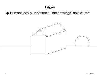
1. Edges • Humans easily understand “line drawings” as pictures.

2. What is an edge? • Edge = where intensity (or color or texture) changes quickly (large gradient) • Step edge • Roof edge • Noisy edge • In 2D, direction of max. gradient is perpendicular to the edge contour

3. Edge Properties • Magnitude • Edge strength (how sharp is the change?) • Direction • Orientation along edge • Perpendicular to gradient (greatest change in brightness) direction

4. Measuring Change • Difference (first derivative - S') • Look for large differences between nearby pixels 1D mask: -1 0 1 (vary # of 0’s) • Thick edges • Maximum absolute value at “center” of edge • Difference of differences (second derivative - S'') • Look for change from growing difference to shrinking difference 1D mask: 1 -2 1 • Value crosses zero at “center” of edge

5. Edge Detection (first derivative) • Roberts (“home” is upper-left, usually) 1 0 0 1 add the results of both 2x2 0 -1 -1 0 convolutions • Sobel (compute “vertical” and “horizontal” separately, take ratio v/h as estimate of tangent of angle of edge, v*v + h*h as estimate of magnitude of edge. 1 2 1 -1 0 1 0 0 0 -2 0 2 -1 -2 -1 -1 0 1 h v

6. Edge Detection (second derivative) • Laplacian – symmetric differences of differences 0 1 0 1 -4 1 4-connected 3x3 0 1 0 1 1 1 1 -8 1 8-connected 3x3 1 1 1 • Laplacian of Gaussian (LoG) (eq. 4.23) • Smooth first, then take second derivative • By properties of convolution, mix into one mask • Also called "Mexican Hat filter” • Difference of Gaussian (DoG) is often a good substitute (as in SIFT paper)

7. Finding the zero-crossing • Look directly for 0’s -- not a good idea (why?) • Look for values near zero -- still not too great? • Look for small regions that contain both positive and negative values - assign one value in the region as zero • Zero-crossing images look like “plate of spaghetti” http://library.wolfram.com/examples/edgedetection/Images/index_gr_87.gif

8. Properties of Derivative Masks • Sum of coordinates of the mask is 0 • Response to uniform region is 0 • Different from smoothing masks, with output = input for uniform region • Response of first-derivative mask is large absolute value at points of high contrast • Positive or negative depending on which side of the edge is dark • Response of second-derivative mask is zero-crossing at points of high contrast

9. Canny Edge Detector • Derived from “first principles” • Detect all edges and only edges (detection) • Put each edge in its proper place (localization) • One detection per edge (one response) • Mathematical optimization for first two, numerical optimization for all three • Assume edges are step edges corrupted by white noise

10. Canny Edge Detector (Algorithm) • Convolve image with Gaussian of scale s • Estimate local edge normal directions for each pixel • Find location of edges using one-dimensional Laplacian • (a form of non-maximal suppression) • Compute edge magnitudes • Threshold edges with hysteresis (as contours are followed) • (two thresholds - general and “border”) • Repeat for multiple scales & find persistent edges

11. Scale • Features exist at different scales • Gaussian smoothing parameter s chooses a scale • Edges can be associated with scale(s) where they appear

12. Choosing Edge Pixels • First (higher threshold) • Find strong edge pixels • Next (lower threshold) • Find (weaker, but not too weak) neighboring edge pixels to follow the contours • This ensures connected edges • Non-maximal suppression • Given directed edges, remove all but the maximum responding pixel in the perpendicular direction to the edge • This effectively thins the edges

13. Color Edges • Detect edges separately in each band (RGB, etc) – combine results for each point • Any edge detector can be used • Depending on combination method, issues can arise • Adding – what if edges cancel? • Or’ing – likelihood of thick edges. • Work in a higher dimension, e.g. 2x2x3 • Estimate local color statistics in each band and make decisions • Estimate magnitudes and orientations in each band, then compute weighted average orientation

14. Contour Following (General) • Assume a list of existing segments, a current segment, and a pixel • Examine every pixel • If "start", create a new segment with this pixel • If "interior", add it to the neighboring segment • If "end", add it to the neighboring segment and end that segment • If "corner", add to IN segment & end that segment, add pixel to OUT segment (or start one, if needed) • If "junction", add to IN segment and end that segment, also add to each OUT segment (creating new ones as necessary)

15. Contour Tracking Issues • Starting a new segment • Adding a pixel to a segment • Need current segment # • Ending a segment • Need current segment # • Finding a junction • Need "in" segment # and "out" segment #s • Finding a corner • Need "in" segment # and "out" segment #

16. Contour Tracking + Thresholding with Hysteresis • Original threshold (high) for selecting initial edge points • Second threshold (lower) for extending contours

17. Encoding Contours • Chain code • Each segment is coded by the direction to its successor (N, NE, E, SE, S, SW, W, NW) • Not amenable to further processing • Arc length parameterization (fig. 4.38) • Curve is “unwrapped”; x and y plotted separately

18. Matching Curves • First normalize: • Scale coordinates so total arc length = 1 • Translate coordinates so centroid is (0,0) • Then match: • Similar curves will have similar coordinates, except • Phase shift due to rotation • Shift in starting point

19. Fitting Lines to Contour • Given a contour (sequence of edgels) • Find a poly-line approximation (sequence of connected line segments) • For which all points lie sufficiently close to the contour. • Example:

20. Curve Approximation Algorithm • Begin with a single segment (the endpoints of the curve) • Repeatedly subdivide the worst-fitting segment until all segments fit sufficiently well • Find the point on the segment furthest from the contour • Split the segment, by creating a new point on the contour. Figure 4.43