
Geometric Transformations
E N D
Presentation Transcript
Geometric Transformations Chun-Yuan Lin CG
Introduction • Now, we tale a look at transformation operations that we can apply to objects to reposition or resize them. • These operations are also used in the viewing routines that convert a world-coordinate scene description to a display for an output device. (geometric transformations) • Geometric transformations can be used to describe how objects might move around in a scene during an animation sequence or simply to view them from another angle. CG
Basic two-dimensional geometric transformations (1) • The geometric transformation functions that are available in all graphics packages are those for translation, rotation and scaling. • We first consider operations in two dimensions, then we discuss how these basic ideas can be extended to three-dimensional scenes. • Two-Dimensional Translation • We perform a translation on a single coordinate point by adding offsets to its coordinates so as to generate a new coordinate position. (multiple coordinate points) • To translate a two-dimensional position, we add translation distance txand ty to the original coordinates (x, y) to obtain the new coordinate position (x’, y’). CG
Basic two-dimensional geometric transformations (2) • The translation distance pair (tx, ty) is called a translation vector or shift vector. • Translate is a rigid-body transformation that moves objects without deformation. (the same before and after the translation) P’ T P CG
Basic two-dimensional geometric transformations (3) • The following routines illustrates the translation operations. class wcPt2D { public: GLfloat x, y; }; void translatePolygon (wcPt2D * verts, GLint nVerts, GLfloat tx, GLfloat ty) { GLint k; for (k = 0; k < nVerts; k++) { verts [k].x = verts [k].x + tx; verts [k].y = verts [k].y + ty; } glBegin (GL_POLYGON); for (k = 0; k < nVerts; k++) glVertex2f (verts [k].x, verts [k].y); glEnd ( ); } CG
Basic two-dimensional geometric transformations (4) • If we want to delete the original polygon, we could display it in the background color before translating it. CG
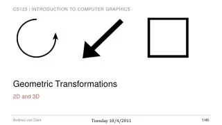
Basic two-dimensional geometric transformations (5) • Two-Dimensional Rotation • We generate a rotation transformation of an object by specifying a rotation axis and a rotation angle. • A two-dimensional rotation of an object is obtained by repositioning the object along a circular path in the xyplane. • Parameters for the two-dimensional rotation are the rotation angle θ and a position (xr, yr) called the rotation point (or pivot point) about which the object is to be rotated. • A positive value defines a counterclockwise rotation. A negative value defines a clockwise rotation. θ yr xr CG
Basic two-dimensional geometric transformations (6) • To simplify the explanation of the basic method, we first determine the transformation equation for rotation of a point position P when the pivot point is at the coordinate origin. (x’, y’) r (x, y) θ r CG
Basic two-dimensional geometric transformations (7) • A column-vector representation for a coordinate position P, as in equation is standard mathematical notation. • OpenGL allows follow the standard column-vector convention. • With a pivot point (xr, yr) : • As with translation rotations are rigid-body transformations that move objects without deformation. (x’, y’) (x, y) (xr, yr) CG
Basic two-dimensional geometric transformations (8) class wcPt2D { public: GLfloat x, y; }; void rotatePolygon (wcPt2D * verts, GLint nVerts, wcPt2D pivPt, GLdouble theta) { wcPt2D * vertsRot; GLint k; for (k = 0; k < nVerts; k++) { vertsRot [k].x = pivPt.x + (verts [k].x - pivPt.x) * cos (theta) - (verts [k].y - pivPt.y) * sin (theta); vertsRot [k].y = pivPt.y + (verts [k].x - pivPt.x) * sin (theta) + (verts [k].y - pivPt.y) * cos (theta); } glBegin {GL_POLYGON}; for (k = 0; k < nVerts; k++) glVertex2f (vertsRot [k].x, vertsRot [k].y); glEnd ( ); } CG
Basic two-dimensional geometric transformations (9) • Two-Dimensional Scaling • To alter the size of an object, we apply a scaling transformation. A simple two-dimensional scaling is performed by multiplying object positions by scaling factors sx and sy to produce the transformed coordinates (x’, y’). • Any positive values can be assigned to the scaling factor sx and sy. • Values less than 1 reduce the size of objects; • Values larger than 1 produce enlargements. • When sx and sy are assigned the same value, a uniform scaling is produced. CG
Basic two-dimensional geometric transformations (10) • Unequal values for sx and sy result in a differential scaling that is often used in design applications. • In some systems, negative values can also be specified for the scaling parameters. This not only resizes an object, it reflects it about one or more of the coordinate axes. • Scaling factors with absolute values less than 1 move objects closer to the coordinate origin. The value larger than 1 move coordinate positions farther from the origin. CG
Basic two-dimensional geometric transformations (11) • We can control the location of a scaled object by choosing a position, called the fixed point (xf, yf), that is to remain unchanged after the scaling transformation. • Objects are now resized by scaling the distances between object points and the fixed point. (xf, yf) CG
Basic two-dimensional geometric transformations (12) class wcPt2D { public: GLfloat x, y; }; void scalePolygon (wcPt2D * verts, GLint nVerts, wcPt2D fixedPt, GLfloat sx, GLfloat sy) { wcPt2D vertsNew; GLint k; for (k = 0; k < n; k++) { vertsNew [k].x = verts [k].x * sx + fixedPt.x * (1 - sx); vertsNew [k].y = verts [k].y * sy + fixedPt.y * (1 - sy); } glBegin {GL_POLYGON}; for (k = 0; k < n; k++) glVertex2v (vertsNew [k].x, vertsNew [k].y); glEnd ( ); } CG
Matrix Representation and Homogenous Coordinates (1) • Many graphics applications involve sequences of geometric transformations. • Here we consider how the matrix representations discussed in the previous sections can be reformulated so that such transformation sequences can be efficiently processed. • We have seen in Section 5-1 that each of the three basic two-dimensional transformation (translation, rotation and scaling) can be expressed in the general matrix form: CG
Matrix Representation and Homogenous Coordinates (2) • Translation • Rotation • Scaling CG
Matrix Representation and Homogenous Coordinates (3) • To produce a sequence of transformation with these equations, such as scaling follow by rotation then translation, we would calculate the transformed coordinates one step at a time. • A more efficient approach, however, is to combine the transformation so that the final coordinate positions are obtained directly from the initial coordinates, without calculating intermediate coordinate values. CG
Matrix Representation and Homogenous Coordinates (4) • Homogeneous Coordinates • Multiplicative and translational terms for a two-dimensional geometric transformation can be combined into a single matrix if we expand the representation to 3 by 3 matrices. • We can use the third column of a transformation matrix for the translation terms, and all transformation equations can be expressed as matrix multiplications. • To expand each two-dimensional coordinate-position representation (x, y) to a three-elements representation (xh, yh, h), called homogeneous coordinates, where the homogenous parameter h is a non-zero value. CG
Matrix Representation and Homogenous Coordinates (5) • Homogenous coordinate representation could be written as (hx, hy, h). • h can be any nonzero value. There are infinite number of equivalent homogenous representations for each coordinate point (x, y). • A convenient choice is simply to set h =1. Each two-dimensional position is then represented with homogenous coordinates (x, y, 1). • When a Cartesian point (x, y) is converted to a homogenous representation (xh, yh, h), equations containing x and y. • Expressing position in homogenous coordinates allows us to represent all geometric transformation equations as matrix multiplications, which is the standard method used in graphics systems. CG
Matrix Representation and Homogenous Coordinates (6) • Two-Dimensional Translation Matrix • We can represent the equations for a two-dimensional translation of a coordinate position using the following matrix multiplication CG
Matrix Representation and Homogenous Coordinates (7) • Two-Dimensional Rotation Matrix • In some graphics libraries, a two-dimensional rotation function generates only rotations about the coordinate origin. A rotation about any other pivot point must then be performed as a sequence of transformation operations. CG
Matrix Representation and Homogenous Coordinates (8) • Two-Dimensional Scaling Matrix CG
Matrix Representation and Homogenous Coordinates (9) • Translation • Rotation • Scaling CG
Inverse Transformations (1) • We obtain the inverse matrix by negating the translation distances. • An inverse rotation is accomplished by replacing the rotation angle by its negative. Negative values for rotation angles generate rotations in a clockwise direction. CG
Inverse Transformations (2) • The inverse matrix for any scaling transformation by replacing the scaling parameters with their reciprocal. CG
Inverse Transformations (3) • Translation • Rotation • Scaling CG
Two-Dimensional Composite Transformations (1) • Using matrix representations, we can set up a sequence of transformations as a composite transformation matrix by calculating the product of the individual transformation. (concatenation, composite of matrices) • It is more efficient to first multiply the transformation matrices to form a single composite matrix. CG
Two-Dimensional Composite Transformations (2) • Composite Two-Dimensional Translations CG
Two-Dimensional Composite Transformations (3) • Composite Two-Dimensional Rotations CG
Two-Dimensional Composite Transformations (4) Composite Two-Dimensional Scaling CG
Two-Dimensional Composite Transformations (5) • Translation • Rotation • Scaling CG
Two-Dimensional Composite Transformations (6) • General Two-Dimensional Pivot-Point Rotation • When a graphics package provides only a rotate function with respet to the coordinate origin, we can generate a two-dimensional rotation about any other pivot point (xr, yr) by performing the following sequence of translate-rotation-translate operations. CG
Two-Dimensional Composite Transformations (7) • General Two-Dimensional Fixed-Point Scaling CG
Two-Dimensional Composite Transformations (8) • Translation • Rotation • Scaling CG
Two-Dimensional Composite Transformations (9) • General Two-Dimensional Scaling Directions • Parameters sxand syscale objects along the x and y directions. We can scale an object in other directions by rotating the object to align the desired scaling directions with the coordinate axes before applying the scaling transformation. y s2 x θ CG s1
Two-Dimensional Composite Transformations (10) • Matrix Concatenation Properties • Multiplication of matrices is associative. • We can construct a composite matrix either by multiplying from left to right or by multiplying from right to left. (for some graphics packages, the order must be specified) • Transformation products may not be commutative. CG
Two-Dimensional Composite Transformations (11) • General Two-Dimensional Composite Transformations and Computational Efficiency • The four elements rsjk are the multiplicative rotation-scaling terms in the transformation, which involve only rotation angles and scaling factors. • Elements trsxand trsy are the translation terms, containing combinations of translation distances, pivot-point and fixed-point coordinates, rotation angles and scaling parameters. CG
Two-Dimensional Composite Transformations (12) • Thus, we need actually perform only four multiplications and four additions to transform coordinate positions. This is the maximum number of computations required for any transformation sequence. • Since rotation calculations require trigonometric evaluations and several multiplications for each transformed point, computational efficiency can become any important consideration in rotation transformations. • When the rotation angle is small, the trigonometric functions can be replaced with approximation values based on the first few terms of their power series expansions. CG
Two-Dimensional Composite Transformations (13) But even with small rotation angles, the accumulated error over many steps can become quite large. Composite transformations often involve inverse matrices. CG
Two-Dimensional Composite Transformations (14) • Two-Dimensional Rigid-Body Transformation • If a transformation matrix includes only translation and rotation parameters, it is a rigid-body transformation matrix. • A rigid-body change in coordinate position is also sometimes referred to as a rigid-motion transformation. • is an orthogonal matrix. CG
Two-Dimensional Composite Transformations (15) • Constructing Two-Dimensional Rotation Matrices • The orthogonal property of rotation matrices is useful for constructing the matrix when we know the final orientation of an object, rather than the amount of angular rotation necessary to put the object into that position. v’ u’ CG
Two-Dimensional Composite Transformations (16) • Two-Dimensional Composite-Matrix Programming Example • A triangle • Scaled with respect to its centroid position • Rotated wth respect to its centroid position • Translate centroid CG
#include <GL/glut.h> #include <stdlib.h> #include <math.h> /* Set initial display-window size. */ GLsizei winWidth = 600, winHeight = 600; /* Set range for world coordinates. */ GLfloat xwcMin = 0.0, xwcMax = 225.0; GLfloat ywcMin = 0.0, ywcMax = 225.0; class wcPt2D { public: GLfloat x, y; }; CG
typedef GLfloat Matrix3x3 [3][3]; Matrix3x3 matComposite; const GLdouble pi = 3.14159; void init (void) { /* Set color of display window to white. */ glClearColor (1.0, 1.0, 1.0, 0.0); } CG
/* Construct the 3 by 3 identity matrix. */ void matrix3x3SetIdentity (Matrix3x3 matIdent3x3) { GLint row, col; for (row = 0; row < 3; row++) for (col = 0; col < 3; col++) matIdent3x3 [row][col] = (row == col); } CG
/* Premultiply matrix m1 times matrix m2, store result in m2. */ void matrix3x3PreMultiply (Matrix3x3 m1, Matrix3x3 m2) { GLint row, col; Matrix3x3 matTemp; for (row = 0; row < 3; row++) for (col = 0; col < 3 ; col++) matTemp [row][col] = m1 [row][0] * m2 [0][col] + m1 [row][1] * m2 [1][col] + m1 [row][2] * m2 [2][col]; for (row = 0; row < 3; row++) for (col = 0; col < 3; col++) m2 [row][col] = matTemp [row][col]; } CG
void translate2D (GLfloat tx, GLfloat ty) { Matrix3x3 matTransl; /* Initialize translation matrix to identity. */ matrix3x3SetIdentity (matTransl); matTransl [0][2] = tx; matTransl [1][2] = ty; /* Concatenate matTransl with the composite matrix. */ matrix3x3PreMultiply (matTransl, matComposite); } CG