Download
1 / 18
190 likes | 210 Vues
Observational tests of an inhomogeneous cosmology. by Christoph Saulder. in collaboration with Steffen Mieske & Werner Zeilinger. A review of basic cosmology. Cosmology applied General Relativity Einstein‘s field equation Cosmological principle: homogeneity and isotropy

E N D
Observational tests of an inhomogeneous cosmology by Christoph Saulder in collaboration with Steffen Mieske & Werner Zeilinger
A review of basic cosmology • Cosmology applied General Relativity • Einstein‘s field equation • Cosmological principle: homogeneity and isotropy • Friedmann-Lemaître-Robertson-Walker metric
Friedmann equations: Written using energy densities: Observed accelerated expansion due to Dark Energy? by NASA
Timescape cosmology • The universe isn’t homogeneous voids and clusters • General relativity is a non-linear theory. • The averaging on large scales has to be modified. • Back reaction from inhomogeneities expected.
Perturbative approach: Buchert‘s scheme (Buchert, 2000) • Perturbation theory alone is not sufficient (Räsänen, 2006) • Importance of local metric, abolishing the universal time parameter in cosmology timescape cosmology (Wiltshire, 2007)
two phase model • Separated by a finite infinity boundary • Walls have a renormalized critical density • Voids are empty • We are in wall environment our observations of the global parameters of the universe have to be recalibrated by Wiltshire, 2007
Nowadays the universe is dominated by voids. • Different expansion rates in different environments due to the local metric. • Voids expand faster than walls • accelerated expansion of the universe (no Dark Energy required anymore) Wiltshire, 2007
Observational features • CMB-power spectrum, cosmic rays, … • different Hubble parameters depending on the environment: void regions expand about 17-22% faster than wall regions • observed Hubble parameter should depend on the foreground (fraction of wall regions in the line of sight) (Schwarz 2010) • effect averages out at the scale of homogeneity
optimal distance between 50 and 200 Mpc • requires redshift and another independent distance indicator, like the fundamental plane • lots of data required • homogenous sample on a large area of the sky: e.g. elliptical galaxies from SDSS • one also has to model the foreground
Data sources • Sloan Digital Sky Survey (SDSS) DR8 • Photometric data (model magnitudes and effective radii in 5 different filters and) • Extinction map (Schlegel et al. 1998) • Spectroscopic data (redshift, central velocity dispersion) • GalaxyZoo (SDSS-based citizen science project for galaxy classification - Lintott et al. 2008 & 2010) • Masses from the (SDSS-based) catalog of groups and clusters by Yang et al., 2008
Performing the test • Recalibrating the fundamental plane • 70000 elliptical galaxies from SDSS • classified by GalaxyZoo (+additional constraints) • redshift range [0 , 0.15] • using a new high quality K-correction (Chilingarian et al. 2010) • RMS in SDSS r-band <10%
Modeling the foreground • Getting positions, redshift based distances of more than 350 000 galaxies from SDSS • Masses from Yang et al. 2008 (SDSS DR4 based) or estimated from mass/light ratios • Homogeneous spheres with a renormalized critical density A part of the foreground model between 100 and 150 h-1 Mpc
Final analysis • Calculate the “individual Hubble-parameters” of a quality selected sample of about 10 000 elliptical galaxies within z < 0.1 using the fundamental plane distances and the redshift from SDSS • Calculate fraction inside finite infinity region by intersecting the spheres with the line of sight to those galaxies. • Compare them and make a plot.
Summary • Using the fundamental plane to calculate distances additional output: new coefficients for the fundamental plane • Comparing distances and redshifts additional output: peculiar motions • The foreground model additional output: masses of clusters and galaxies + peculiar motions
Testing timescape cosmology • First results look promising, but there are still several open problems in our models. • Positive results would be a major discovery. • Intermediate results would favor Dark Energy theories with a Chameleon effect such as f(R) modified gravity. • Negative results would support the -CDM. CAST LIGHT ON DARK ENERGY