Lecture 7: Wireless Ad-Hoc Networks

1. Lecture 7: Wireless Ad-Hoc Networks

2. Wireless Ad-hoc Networks • Network without infrastructure • Use components of participants for networking • Examples • Single-hop: All partners max. one hop apart • Bluetooth piconet, PDAs in a room,gaming devices… • Multi-hop: Cover larger distances, circumvent obstacles • Bluetooth scatternet, TETRA police network, car-to-car networks… • Internet: MANET (Mobile Ad-hoc Networking) group

3. Mobile Router Manet Mobile Devices Mobile IP, DHCP Fixed Network Router End system Manet: Mobile Ad-hoc Networking

4. Routing • Goal: determine “good” path (sequence of routers) thru network from source to dest • Global information: • all routers have complete • Topology, link cost info • “link state” algorithm • Decentralized: • router knows physically-connected neighbors, link costs to Neighbors • routers exchange of info with neighbors • Distance vector routing: the routing table is constructed from a distance vector at each node • routing table (at each host): the next hop for each destination in the network

5. Distance Vector Routing Distance vector at node E D (E,D,C) c(E,D) + shortest(D,C) ==2+2 = 4 D (E,D,A) c(E,D) + shortest(D,A) ==2+3 = 5 D (E,B,A) c(E,B) + shortest(B,A) ==8+6 = 14

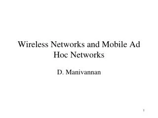
6. Routing Problem • Highly dynamic network topology • Device mobility plus varying channel quality • Separation and merging of networks possible • Asymmetric connections possible N7 N6 N6 N7 N1 N1 N2 N3 N2 N3 N4 N4 N5 N5 good link weak link time = t2 time = t1

7. Traditional routing algorithms • Distance Vector • periodic exchange of messages with all physical neighbors that contain information about who can be reached at what distance • selection of the shortest path if several paths available • Link State • periodic notification of all routers about the current state of all physical links • router get a complete picture of the network • Example • ARPA packet radio network (1973), DV-Routing • every 7.5s exchange of routing tables including link quality • updating of tables also by reception of packets • routing problems solved with limited flooding

8. Routing in Ad-hoc Networks • THE big topic in many research projects • Far more than 50 different proposals exist • The most simplest one: Flooding! • Reasons • Classical approaches from fixed networks fail • Very slow convergence, large overhead • High dynamicity, low bandwidth, low computing power • Metrics for routing • Minimal • Number of nodes, loss rate, delay, congestion, interference … • Maximal • Stability of the logical network, battery run-time, time of connectivity …

9. Problems of Traditional Routing Algorithms • Dynamic of the topology • frequent changes of connections, connection quality, participants • Limited performance of mobile systems • periodic updates of routing tables need energy without contributing to the transmission of user data, sleep modes difficult to realize • limited bandwidth of the system is reduced even more due to the exchange of routing information • links can be asymmetric, i.e., they can have a direction dependent transmission quality

10. Distance Vector Routing • Early work • on demand version: AODV • Expansion of distance vector routing • Sequence numbers for all routing updates • assures in-order execution of all updates • avoids loops and inconsistencies • Decrease of update frequency • store time between first and best announcement of a path • inhibit update if it seems to be unstable (based on the stored time values)

11. D A Link 2 Link 4 C Link 1 Link 6 B Link 3 Link 5 E Distance Vector Routing • Consider D • Initially nothing in routing table. • When it receives an update from C and E, it notes that these nodes are one hop away. • Subsequent route updates allow D to form its routing table.

12. D A Link 2 Link 4 Broken C Link 1 Link 6 Broken B Link 3 Link 5 E Network partitions into two isolated islands Destination Sequenced Distance Vector (DSDV) • Disadvantage of Distance Vector Routing is formation of loops. • Let Link 2 break, and after some time let link 3 break.

13. Destination Sequenced Distance Vector (DSDV) • After Link 2 is broken, Node A routes packets to C, D, and E through Node B. • Node B detects that Link 3 is broken. • It sets the distance to nodes C, D and E to be infinity. • Let Node A in the meantime transmit a update saying that it can reach nodes C, D, and E with the appropriate costs that were existing before – i.e., via Node B. • Node B thinks it can route packets to C, D, and E via Node A. • Node A thinks it can route packets to C, D, and E, via Node B. • A routing loop is formed – Counting to Infinity problem. • Methods that were proposed to overcome this

14. Destination Sequenced Distance Vector (DSDV) D A Broken Link 4 Link 2 C Link 1 Link 6 Broken B Link 3 Link 5 E Network partitions into two isolated islands Each routing table entry is tagged with a “sequence number” that is originated by the corresponding destination node in that entry. • Node A’s update is stale !!! Sequence number indicated for nodes C,D, and E is lower than the sequence number maintained at B. Looping avoided !

15. Dynamic Source Routing I • Split routing into discovering a path and maintaining a path • Discover a path • only if a path for sending packets to a certain destination is needed and no path is currently available • Maintaining a path • only while the path is in use one has to make sure that it can be used continuously • No periodic updates needed!

16. Dynamic Source Routing II • Path discovery • broadcast a packet with destination address and unique ID • if a station receives a broadcast packet • if the station is the receiver (i.e., has the correct destination address) then return the packet to the sender (path was collected in the packet) • if the packet has already been received earlier (identified via ID) then discard the packet • otherwise, append own address and broadcast packet • sender receives packet with the current path (address list) • Optimizations • limit broadcasting if maximum diameter of the network is known • caching of address lists (i.e. paths) with help of passing packets • stations can use the cached information for path discovery (own paths or paths for other hosts)

17. DSR: Route Discovery P R Sending from C to O C G Q B I E M O K A H L D N F J

18. DSR: Route Discovery P R Broadcast [O,C,4711] C Q G [O,C,4711] B I E M O K A H L D N F J

19. DSR: Route Discovery P R [O,C/G,4711] C Q G [O,C/G,4711] [O,C/B,4711] B I E M O K A H [O,C/E,4711] L D N F J

20. DSR: Route Discovery P R C Q G [O,C/G/I,4711] B I E M O K A H [O,C/E/H,4711] L D [O,C/B/A,4711] N F J [O,C/B/D,4711] (alternatively: [O,C/E/D,4711])

21. DSR: Route Discovery P R C Q G B I [O,C/G/I/K,4711] E M O K A H L D N F J [O,C/E/H/J,4711] [O,C/B/D/F,4711]

22. DSR: Route Discovery P R C Q G B I [O,C/G/I/K/M,4711] E M O K A H L D N F J [O,C/E/H/J/L,4711] (alternatively: [O,C/G/I/K/L,4711])

23. DSR: Route Discovery P R C Q G B I E M O K A H L D N F J [O,C/E/H/J/L/N,4711]

24. DSR: Route Discovery P R C Q G Path: M, K, I, G B I E M O K A H L D N F J

25. Dynamic Source Routing III • Maintaining paths • after sending a packet • wait for a layer 2 acknowledgement (if applicable) • listen into the medium to detect if other stations forward the packet (if possible) • request an explicit acknowledgement • if a station encounters problems it can inform the sender of a packet or look-up a new path locally

26. neighbors (i.e. within radio range) Interference-based routing • Routing based on assumptions about interference between signals N1 N2 R1 S1 N3 N4 N5 N6 R2 S2 N9 N8 N7

27. Examples for Interference based Routing • Least Interference Routing (LIR) • calculate the cost of a path based on the number of stations that can receive a transmission • Max-Min Residual Capacity Routing (MMRCR) • calculate the cost of a path based on a probability function of successful transmissions and interference • Least Resistance Routing (LRR) • calculate the cost of a path based on interference, jamming and other transmissions • LIR is very simple to implement, only information from direct neighbors is necessary

28. A Plethora of Ad Hoc Routing Protocols • Flat • proactive • FSLS – Fuzzy Sighted Link State • FSR – Fisheye State Routing • OLSR – Optimized Link State Routing Protocol (RFC 3626) • TBRPF – Topology Broadcast Based on Reverse Path Forwarding • reactive • AODV – Ad hoc On demand Distance Vector (RFC 3561) • DSR – Dynamic Source Routing (RFC 4728) • DYMO – Dynamic MANET On-demand • Hierarchical • CGSR – Clusterhead-Gateway Switch Routing • HSR – Hierarchical State Routing • LANMAR – Landmark Ad Hoc Routing • ZRP – Zone Routing Protocol • Geographic position assisted • DREAM – Distance Routing Effect Algorithm for Mobility • GeoCast – Geographic Addressing and Routing • GPSR – Greedy Perimeter Stateless Routing • LAR – Location-Aided Routing

29. Further Difficulties and Research Areas • Auto-Configuration • Assignment of addresses, function, profile, program, … • Service discovery • Discovery of services and service providers • Multicast • Transmission to a selected group of receivers • Quality-of-Service • Maintenance of a certain transmission quality • Power control • Minimizing interference, energy conservation mechanisms • Security • Data integrity, protection from attacks (e.g. Denial of Service) • Scalability • 10 nodes? 100 nodes? 1000 nodes? 10000 nodes? • Integration with fixed networks

30. Clustering of Ad-hoc Networks Internet Cluster head Base station Cluster Super cluster