Adaptivity with Moving Grids
240 likes | 364 Vues
This talk, presented by Santhanu Jana, explores the concept of adaptivity in moving grids, focusing on techniques for grid movement and their implications in solving time-dependent partial differential equations (PDEs). The motivation behind this work includes applications in various fields such as physics, fluid-structure interactions, aeroacoustics, and simulations of dynamic processes like crystal growth and heart modeling. The presentation covers Lagrangian, Eulerian, and mixed methods for grid adaptation, highlighting their advantages, challenges, and necessary modifications in conservation equations, ensuring a comprehensive understanding of moving grid methodologies.

Adaptivity with Moving Grids
E N D
Presentation Transcript
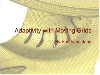
Adaptivity with Moving Grids By Santhanu Jana
Talk Overview • Motivation • Techniques in Grid Movement • Physical and Numerical Implications in time dependent PDE‘s • Outlook and Conclusions
Motivation • Applications in Physics • Fluid Structure • Aerostructures and Aeroacoustics • Moving Elastic Structures eg. Simulation of Heart • Thermodynamical Considerations • Phase Change Phenomena • Free Surfaces • Material Deformations • Multiphase Flows
Some Examples-Fluid Structure Interactions Source:http://www.onera.fr/ddss-en/aerthetur/aernummai.html :http://www.erc.msstate.edu/simcenter/04/april04.html
Some Examples-Phase Change Phenomena Crystal Growth Source: Work At LSTM
What Is Moving Grid ? • PDE’s must be satisfied on each side of the interface (often different equations on each side) • Solutions coupled through relationships or jump conditions that must hold at the interface • These conditions may be in the form of differential equations • Movement of the interface is unknown in advance and must be determined as part of the solution
Computational Techniques in Moving Grids • Lagrangian Methods • Eulerian Methods • Mixed Lagrangian and Eulerian Methods
Lagrangian Methods(1) • Explicit Tracking of the Interface Boundary • No Smearing of Information at the boundary • No Modeling is necessary to define the interface • Un/structured boundary Conforming Grids • No modelling to define the interface • Grid Regeneration • Grid Adaption • Requires redistribution of field information
Problems in Lagrangian Methods(2) • Grid Distortion • Solution: Grid Sliding
Problems in Lagrangian Methods(3) • Resolving Complex Structures near the interface • Solution: Local Grid Refinement • Increase the Convergence order
Necessary Modifications in the Conservation Equations(4) • Eg: Solution of Navier Stokes Equations 1 ) Momentum Equation: 2 ) Energy Equation: 3 ) Mass Conservation Equation:
Necessary Modifications in the Conservation Equations(5) 4) Geometric Conservation NOTE: Grid Velocities should satisfy Geometric Conservation Equation References: 1) Thomas, P.D., and Lombard, C.K., Geometric Conservation Law and Its Applications to Flow Computations on Moving Grids," AIAA Journal, Vol. 17, No. 10, pp. 1030-1037. 2) Weiming Caso, Weizhang Huang and Robert D. Russel A Moving mesh Method based on the Geometric Conservation Law, SIAM J. SCI. COMPUTING Vol24, No1, pp.118-142
Eulerian Methods(1) • Boundary is derived from a Field Variable eg: VOF, Level Set • Interface is diffused and occupies a few grid cells in practical calculations • Strategies are necessary to sharpen and physically reconstruct the interface • Boundary Conditions are incorporated in the governing PDE. • Grid Generation: Grid is created once
Basic Features of Eulerian Methods(2) • Grid Topology remains simple even though the interface may undergo large deformations • Two Basic Approaches • Immersed Boundary Method • Without explicit tracking • Interface Cut-Cell Method • Interface tracked explicitly (Reconstruction procedures to calculate coefficients in the Solution Matrix) Ref: 1) C.S.Peskin, Numerical Analysis of blood flow in the heart, Journal of Computational Physics, 25, (1977), 220-252 2) H.S.Udaykumar, H.C.Kan, W.Shyy, and R.Tran-Son-Tay, Multiphase dynamics in arbitrary geometries on fixed cartesian grids, Journal of Computational Physics, 137, (1997), 366-405
ds FLUID 2 FLUID I n Eulerian Methods: Immersed Boundary Method (3) The Interface between Fluid 1 and Fluid 2 is represented by curve C is marked by particles (dots) that do not coincide with the grid nodes C Important Considerations: • Interface Representation • Assignment of Material Properties (Change of Contants in PDE) • Immersed Boundary Treatment Marker Particles
Immersed Boundary Method: Interface Representation(4) • Immersed boundary represented by C(t) • Curve in 2D and Surface in 3D. • Markers or interfacial points of coordinates • Markers are regularly distributed along C(t) at a fraction of grid spacing (ds). • The interface is parameterised as a function of arclength by fitting a quadratic polynomial. • The normal vector and curvature (divergence of normal vector) is evaluated.
Immersed Boundary Method: Material Properties(5) • Assign in each fluid based on some step function • Should handle the transition zone. • Treatment handles improved Numerical Stability and solution smothness
Immersed Boundary Method: Boundary Treatment(6) • Facilitates Communication between the moving markers (interface) and the fixed grid. • Evaluation of the forces acting on the interface • Estimation of interface velocity • Advection of the interface. • To improve accuracy of the interface tracking, a local grid refinement aroung the interface can be used. Ref: H. S. Udaykumar, R. Mittal, P. Rampunggoon and A. Khanna,A Sharp Interface Cartesian Grid Method for Simulating Flows with Complex Moving Boundaries Journal of Computational Physics, Volume 174, Issue 1, 20 November 2001, Pages 345-380
Interface Cut Cell Method(6) Improvement over Immersed Boundary method : Summary of the Procedure • Location of Interface Marker. • The interfacial marker closest to mesh point. • Material parameters. • Interface Cell Reconstruction : Geometric details. • Intersection of the immersed boundary with the Fixed grid mesh. • Suitable stencil and evaluate coefficients Example: Stencil to evaluate variables
Mixed Eulerian-Lagrangian methods • Combines features of Eulerian and Lagrangian methods. • Solver doesnot see discontinuity (Eulerian Methods) • Solver experiences distributed forces and material properties on the vicinity of the interface • No smearing of interface Ref: S. Kwak and C. Pozrikidis Adaptive Triangulation of Evolving, Closed, or Open Surfaces by the Advancing-Front Method Journal of Computational Physics, Volume 145, Issue 1, 1 September 1998, Pages 61-88
Outlook and Conclusion • Lagrangian Methods are physically consistent over Eulerian Methods but suffers when grid distortion is severe. • In Eulerian Methods mergers and break ups are tackled automatically. • Interface Reconstruction in Eulerian Methods may be very complicated on nonorthogonal un/structured grid. Extension to 3D might be a problem. • Local Refinement may be used to the capture the interface more accurately.