Download
1 / 18
180 likes | 302 Vues
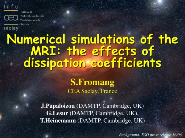
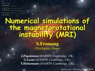
Numerical simulations of the magnetorotational instability (MRI). S.Fromang CEA Saclay, France J.Papaloizou ( DAMTP, Cambridge, UK) G.Lesur ( DAMTP, Cambridge, UK), T.Heinemann (DAMTP, Cambridge, UK). Background: ESO press release 36/06. The magnetorotational instability.

E N D
Numerical simulations of the magnetorotational instability (MRI) S.Fromang CEA Saclay, France J.Papaloizou (DAMTP, Cambridge, UK) G.Lesur (DAMTP, Cambridge, UK), T.Heinemann (DAMTP, Cambridge, UK) Background: ESO press release 36/06
The magnetorotational instability (Balbus & Hawley, 1991) nonlinear evolution numerical simulations
The shearing box (1/2) r x y H H z y H x • Local approximations • Ideal MHD equations + EQS (isothermal) • vy=-1.5x • Shearing box boundary conditions (Hawley et al. 1995)
The shearing box (2/2) z x Transport diagnostics • Maxwell stress: TMax=<-BrB>/P0 • Reynolds stress: TRey=<vrv>/ P0 • =TMax+TRey rate of angular momentum transport Magnetic field configuration Zero net flux: Bz=B0 sin(2x/H) Net flux: Bz=B0
The 90’s and early 2000’s Local simulations (Hawley & Balbus 1992) • Breakdown into MHD turbulence (Hawley & Balbus 1992) • Dynamo process (Gammie et al. 1995) • Transport angular momentum outward: <>~10-3-10-1 • Subthermal B field, subsonic velocity fluctuations BUT: low resolutions used (323 or 643)
The issue of convergence (Nx,Ny,Nz)=(64,100,64) Total stress: =4.2 10-3 (Nx,Ny,Nz)=(128,200,128) Total stress: =2.0 10-3 (Nx,Ny,Nz)=(256,400,256) Total stress: =1.0 10-3 Fromang & Papaloizou (2007) ZEUS code (Stone & Norman 1992), zero net flux The decrease of with resolution is not a property of the MRI. It is a numerical artifact!
Dissipation Small scales dissipation important Explicit dissipation terms needed (viscosity & resistivity) • Reynolds number: Re =csH/ • Magnetic Reynolds number: ReM=csH/ Magnetic Prandtl number Pm=/
Case I Zero net flux
Pm=/=4, Re=3125 ZEUS PENCIL CODE SPECTRAL CODE NIRVANA Fromang et al. (2007) ZEUS : =9.6 10-3 (resolution 128 cells/scaleheight) NIRVANA :=9.5 10-3 (resolution 128 cells/scaleheight) SPECTRAL CODE: =1.0 10-2 (resolution 64 cells/scaleheight) PENCIL CODE :=1.0 10-2 (resolution 128 cells/scaleheight) Good agreement between different numerical methods
Pm=/=4, Re=6250 (Nx,Ny,Nz)=(256,400,256) Density Vertical velocity By component Movie: B field lines and density field (software SDvision, D.Polmarede, CEA)
Effect of the Prandtl number Pm=/=4 Pm=/= 8 Pm=/= 16 Pm=/= 2 Pm=/= 1 Take Rem=12500 and vary the Prandtl number…. (Lx,Ly,Lz)=(H,H,H) (Nx,Ny,Nz)=(128,200,128) • increases with the Prandtl number • No MHD turbulence for Pm<2
The Pm effect Pm =/ <<1 Viscous length << Resistive length Schekochihin et al. (2004) Velocity Magnetic field Velocity Magnetic field Schekochihin et al. (2007) Schekochihin et al. (2007) Pm=/>>1 Viscous length >> Resistive length • No proposed mechanisms…but: • Dynamo in nature (Sun, Earth) • Dynamo in experiments (VKS) • Dynamo in simulations
Parameter survey Pm ? MHD turbulence ? No turbulence Re • Small scales important in MRI turbulence • Transport increases with the Prandtl number • No transport when Pm≤1 For a given Pm, does α saturates at high Re?
Pm=4, Transport Re=3125 Re=6250 Re=12500 (Nx,Ny,Nz)=(128,200,128) (Nx,Ny,Nz)=(256,400,256) (Nx,Ny,Nz)=(512,800,512) Total stress =9.2 ± 2.8 10-3 Total stress =7.6 ± 1.7 10-3 Total stress =2.0 ± 0.6 10-2 No systematic trend as Re increases…
Case II Vertical net flux
Influence of Pm - Pseudo-spectral code, resolution: (64,128,64) - (Lx,Ly,Lz)=(H,4H,H) - =100 Lesur & Longaretti (2007)
Conclusions & open questions Pm MHD turbulence ? No turbulence Re • Include explicit dissipation in local simulations of the MRI: • resistivity AND viscosity • Zero net flux AND nonzero net flux • an increasing function of Pm • Behavior at large Re is unclear • Global simulations? What is the effect of large scales? • State of PP disks very uncertain (Pm<<1) • Dead zone location/structure very uncertain…