Earth Radiation Budget
Earth Radiation Budget. Satellite Remote Sensing II - ATS 770 Presentation3 October 26 th , 2011. By Nan Feng Department of Atmospheric Sciences The University of Alabama in Huntsville Huntsville, AL. Outline. Introduction Uncertainties Angular Distribution Models (ADM) Validations

Earth Radiation Budget
E N D
Presentation Transcript
Earth Radiation Budget Satellite Remote Sensing II - ATS 770 Presentation3 October 26th, 2011 By Nan Feng Department of Atmospheric Sciences The University of Alabama in Huntsville Huntsville, AL
Outline • Introduction • Uncertainties • Angular Distribution Models (ADM) • Validations • Conclusion
Introduction to Earth’s Radiation Budget • Absorption of Insolation and Emission of terrestrial radiation drive the General Circulation of the Atmosphere
Introduction to Earth’s Radiation Budget Largely responsible for Earth’s weather and climate
IPCC report 2007 Medium-Low Level Understanding
Direct and indirect effects of tropospheric aerosols Increased planetary albedo: Scattering solar COOLING! Sun Decreased planetary albedo: Absorbing solar WARMING! Impact clouds and precipitation processes COMPLICATED! Surface
Aerosol climate impact • Direct effects • Scattering solar energy • Absorbing solar/terrestrial energy • Indirect effects (Modify cloud properties) • More droplets----clouds are brighter (Twomey, 1977 ) • More droplets----longer cloud life time (Albrecht,1989) • Semi-direct effect • Absorbing aerosols heat airs and evaporate clouds (Hansen et al., 1997) ARF Estimation Aerosol Radiative Forcing = FCLEAR-SKY – FAEROSOL
How can we study earth radiation budget ? • Global Climate Models • Global Observations • Satellite measurements of radiative quantities.
Spectral Categories Instruments for Radiation budget : • Narrowband Sensors • Broadband Sensors • Field of View Categories : • Wide field-of-view (WFOV) Nonscanner • - Often called FLAT-PLATE sensors • - Measure radiation horizon to horizon • - 120o angular resolution • - Example : Nimbus7 ERB, ERBE, CERES • - Longer lifetime due to less wear • Narrow field-of-view (NFOV) Scanner - AVHRR, Nimbus 6,7 ERB, ERBE, CERES
The Goddard Space Flight Center built the Earth Radiation BudgetSatellite (ERBS) on which the first ERBE instruments were launched by the Space Shuttle Challenger in 1984. ERBE instruments were also launched on two National Oceanic and Atmospheric Administration weather monitoring satellites, NOAA 9 and NOAA 10 in 1984 and 1986. Both had two instruments : Scanner & Non-Scanner http://eosweb.larc.nasa.gov/PRODOCS/erbe/table_erbe.html
CERES SCAN MODES Unique feature! Rotating Azimuth Plane Cross-Track Scan mode
CERES Spatial Coverage CERES Scan Modes
Design Specifications • Orbits: 705 km altitude, 10:30 a.m. descending node (Terra) or 1:30 p.m. ascending node (Aqua), • sun-synchronous, near-polar; • 350 km altitude, 35° inclination (TRMM) • Spectral Channels: • Shortwave : 0.3 - 5.0 µmWindow: 8 - 12 µm Total: 0.3 to 200 µm • Swath Dimensions: Limb to limb • Angular Sampling: Cross-track scan and 360° azimuth biaxial scan • Spatial Resolution: 20 km at nadir (10 km for TRMM)
CERES has four main objectives: • Provide a continuation of the ERBE record of radiative fluxes at the top of the atmosphere (TOA) , analyzed using the same algorithms that produced the ERBE data • Double the accuracy of estimates of radiative fluxes at TOA and the Earth's surface • Provide the first long-term global estimates of the radiative fluxes within the Earth's atmosphere • Provide cloud property estimates that are consistent with the radiative fluxes from surface to TOA
Limitations: • Inadequate diurnal variation, only twice daily observations (diurnal problem) • Satellite sensors do not measure exactly the wavelength integrated radiation budget quantities (spectral correction problem or unfiltering problem) • Radiance-to-flux conversion (angular dependence problem)
The uncertainties of ERB studies • Radiance calibration • Filtered to Unfiltered Radiances • Cloud contamination • Clear Sky Estimation • Radiances to flux Conversion - ADM
Radiance to Flux Conversion Isotropic Scattering • Satellite measures radiance (I(o,,))at a given sun-satellite geometry during overpass • This radiance must be converted to flux • If surface is Lambertian, then for isotropic scattering, flux F(o) = π * I(o,,) • However, for non-lambertian surfaces, the scattering is not isotropic Anisotropic Scattering Backward Forward
Radiance to Flux Conversion • Angular measurements can be integrated to obtain non-Lambertian flux (F(o)) • Anisotropic factor or angular distribution model = The Ratio of the Lambertian flux to non-Lambertian flux • ADM = Ratio of equivalent Lambertian flux to actual flux • R(o,,)= π*I(o,,)/ F(o)
ADMs (Sorting-into-Angular-Bins, SABs) Large ensemble of radiance measurements are first sorted into discrete angular bins and parameters that define an ADM scene type and ADM anisotropic factors for a given scene type(j) are given by where : is the average radiance (corrected for Earth-sun distance in the SW) in an angular bin , is the upwelling flux in a solar zenith angle bin, which is determined by directly integrating over all angles (Loeb et al., 2003). The set of angles oi, k, and .
Examples ADMs as the function of 0.55 0.55: 0.0-0.1 0.55:0.1-0.2 0.55: 0.2-0.4 < 0.6 0.55: 0.2-0.4 > 0.6 Glint
ADM Scene Identification • The main reason for defining ADMs by scene type is to reduce the error in the albedo estimate. • Earth scenes have distinct anisotropic characteristics which depend on their physical and optical properties. (e.g. thin vs thick clouds; cloud-free, broken, overcast, etc.) • Scene identification must be self-consistent. Biases in cloud property retrievals (e.g. due to 3D cloud effects) should not introduce biases in flux/albedo estimates.
CERES Single Scanner Footprint (SSF) Product • Coincident CERES radiances and imager-based cloud and aerosol properties • Use VIRS (TRMM) or MODIS (Terra or Aqua) to determine following in up to 2 cloud layers over every CERES FOV: • Macrophysical: Factional coverage, Height, Radiating Temperature, Pressure • Microphysical: Phase, Optical Depth, Particle Size, Water Path • Clear Area: Albedo, Skin Temperature, Aerosol optical depth
TRMM ADMs • Better scene identification and Increased ADM sensitivity to anisotropy • using collocated VIRS and CERES data. • VIRS is a narrowband imager – 2km spatial resolution • CERES has footprint of 10km (TRMM) at nadir • 200 shortwave and 100 longwavescene types http://asd-www.larc.nasa.gov/Inversion Loeb et al., 2003; JAM, 42, 240-265 Loeb et al., 2003; JAM, 42, 1748-1769
Comparisons between TRMM and Terra CERES • TRMM • Only 9 months of data (Jan-Aug, 1998 + March 2000) • Spatial coverage limited to ±38o only • 350 km precessing orbit with 35o inclination 46 days for full range of SZA • land cover types = only 4 categories based on IGBP • TERRA • global coverage • increased sampling • Data available since 2000 • need for new ADMs because spatial resolution and geographic coverage different
CERES Terra SW ADMs – (a) Ocean – (1) Clear Conditions: MODIS pixel-level cloud cover fraction less or equal than 0.1% Instantaneous TOA fluxes are determined using combination of empirical and theoretical ADMs as follows: is determined from wind speed-dependent empirical ADMs that are derived from CERES data are theoretical radiative transfer model anisotropic factors evaluated at the measured CERES radiance and mean CERES radiance in a given ADM angular bin, respectively.
SW ADMs – (a) Ocean – (2) Clouds Continuous ADMs using analytical functions that relate CERES radiances and imager parameters (e.g. cloud fraction and cloud optical depth.) Where, is the retrieved Cloud optical depth of the ith Pixel within the CERES FOV • Try to combine f and • into a single parameter • Third order polynomial • Five paras sigmoidal fit
SW ADMs – (a) Ocean – (2) Clouds Continuous ADMs using analytical functions that relate CERES radiances and imager parameters (e.g. cloud fraction and cloud optical depth.) The sigmoidal fit relative errorremains less than 1% in every cloudfraction interval The polynomial fit relative errorreaches -3% at intermediate cloud fractions Similar results are obtained when other angular bins are considered or when separate fits are derived for mixed-phased and ice clouds. The close relationship btw SW radiance and occurs in spite of the rather large range of cloud properties associated with a given range In general, the rms error in predicting instaneous SW radiances using the sigmoidal fit is btw 5% and 10%.
SW ADMs – (a) Ocean – (2) Clouds Continuous ADMs using analytical functions that relate CERES radiances and imager parameters (e.g. cloud fraction and cloud optical depth.)
SW ADMs – (a) Ocean – (2) Clouds In each solar zenith angle interval, the liquid water clouds show well-defined peaks in anisotropy for = - 30 to -60 and close to nadir due to the cloud glory and rainbow features, while peaks in anisotropy occur for ice clouds between = 30 to 60 in the specular reflection direction, also observed by Chefer et al. (1999) in POLDER measurements. Likely due to horizontally oriented ice crystals.
ADMs for Terra CERES: • 1. Shortwave: • Clear Land: Stratify by IGBP type + vegetation index + taer • 1×1 latitude and longitude equal area regions with a temporal resolution of 1 month • Clouds over Land: Continuous scene type using sigmoidal functional fits to data. • Clear Snow/ice: Stratify by NDSI (permanent snow, fresh snow, or sea ice. Further stratified into ‘bright’ and dark subclasses) • Clouds over Snow: greater dependence on vza than cloud free scence. • 2. Longwave and Window: • Cloud-free conditions: more surface types and high angular bins resolutions (Stratified by precipitable water, imager-based surface skin temperature and etc.) • Cloudy conditions: a function of precipitable water, surface and cloud top temperature, surface and cloud top emissivity and cloud fraction.
Terra ADMs • Improvements : • using collocated MODIS and CERES data. • MODIS is a multispectral (36) imager with • 250m, 500m, 1km spatial resolution • CERES has footprint of 20 km (Terra, Aqua) at nadir • scene type information from MODIS • angular bin resolution sharpened to 2o in shortwave • wind-speed resolution (over ocean) increase to 2 m/s • over land, ADMs built for 1ox1o lat-lon regions at 1 month temporal resolution • NDVI used to separate sub-regions within 1ox1o regions
Terra CERES ADMs: Validation • A series of consistency tests are performed to evaluate uncertainties in TOA fluxes derived with the CERES SW and LW ADMs: • Regional Mean TOA Flux Error Test (SW, LW and WN) • Instantaneous TOA Flux Uncertainties Test • Comparisons with ERBE-Like TOA Fluxes • Comparison with radiative transfer model
Regional Mean TOA Flux Error (Direct Integration) • Regionally averaged ADM-derived TOA fluxes are compared with regional mean fluxes obtained by direct integration of observed mean radiances (DI fluxes). • regions of 10×10 latitude and longitude, over several months. • The regional all-sky ADM is constructed by sorting the radiances in a region by viewing geometry (,0 ,) and evaluating the ratio of the mean radiance in an angular bin to the DI flux, obtained by integrating radiances in all angular bins.
Instantaneous TOA Flux Uncertainties Test • Compare ADM-derived TOA fluxes over 1 regions from different viewing geometries. • Comparing CERES Terra ADMs and surface observations (Programmable Azimuth Plane Scans Over ARM-SGP TEST) • Terra-Aqua Instantaneous TOA Flux Comparison over Greenland (69.5N) • Multi-angle TOA Flux Consistency Tests (Merged dataset of MISR-MODIS-CERES)
Instantaneous TOA Flux Uncertainties Test Clear-sky multiangle SW TOA flux consistency: (a) Relative difference [F(=50-60) –F(Nadir)]/F(Nadir); (b) Relative RMS difference
Validation results: • Based on all results and a theoretically derived conversion btw TOA flux consistency and TOA flux error, the best estimate of the error in CERES TOA flux due to the radiance-to-flux conversion is 3% (10Wm-2) in the SW and 1.8% (3 to 5 Wm-2) in the LW. • Monthly mean TOA fluxes based on ERBE ADMs are larger than monthly mean TOA fluxes based on CERES Terra ADMs by 1.8 Wm-2and 1.3Wm-2in the SW and LW, respectively.
To summary • The Angular Characteristics of TOA Radiance depends on • Viewing Geometry [Loeb et al., 2002; Suttles et al., 1988] • Surface characteristics (snow is brighter than vegetation) [Loeb et al., 2002; Suttles et al., 1988] • Atmospheric Characteristics (clouds, aerosols) [Loeb et al., 2002; Li et al., 2000; Zhang et al., 2005; Falguni et al., 2011] • Current CERES ADMs = f(geometry, surface, clouds)
References • Leob, N.G., N.M. Smith, S. Kato, W.F. Miller, S.K.Gupta, P.Minnis, and B.A. Wielicki, 2003: Angular distribution models for top-of-atmosphere radiative flux estimation from the Clouds and the Earth’s Radiant Energy System instrument on the Tropical Rainfall Measuring Satellite. Part I: Methodology. J. Appl. Meteor., 42, 240-265. • Leob, N.G., S. Kato, K. Loukachine, and N.M. Smith (2005), Angular distribution models for top-of-atmosphere radiative flux estimation from the Clouds and the Earth's Radiant Energy System instrument on the Terra satellite. Part I: Methodology, J.Atmos. Oceanic. Technol., 22, 338-351 • Loeb, N. G., Kato, S. et al., Angular Distribution Models for Top-of-Atmosphere Radiative Flux Estimation from the Clouds and the Earth’s Radiant Energy System Instrument on the Terra Satellite. Part II: Validation, American Meteorological Society DOI: 10.1175/JTECH1983.1, 2007
Filtered to unfiltered radiance • Radiometric count conversion algorithms convert the detector digital count into filtered radiances. • For use in science applications, radiances from earth scenes should be independent of the optical path in the instrument.
Filtered To Unfiltered Radiance Unfiltered radiance Filtered radiance Conversion