Evolutionary Game Theory
490 likes | 695 Vues
Evolutionary Game Theory. Amit Bahl CIS620. Outline. EGT versus CGT Evolutionary Stable Strategies Concepts and Examples Replicator Dynamics Concepts and Examples Overview of 2 papers Selection methods, finite populations . EGT v. Conventional Game Theory.

Evolutionary Game Theory
E N D
Presentation Transcript
Evolutionary Game Theory Amit Bahl CIS620
Outline • EGT versus CGT • Evolutionary Stable Strategies Concepts and Examples • Replicator Dynamics Concepts and Examples • Overview of 2 papers Selection methods, finite populations
EGT v. Conventional Game Theory • Models used to study interactive decision making. • Equilibrium is still at heart of the model. • Key difference is in the notion of rationality of agents.
Agent Rationality • In GT, one assumes that agents are perfectly rational. • In EGT, trial and error process gives strategies that can be selected for by some force (evolution - biological, cultural, etc…). • This lack of rationality is the point of departure between EGT and GT.
Evolution • When in biological sense, natural selection is mode of evolution. • Strategies that increase Darwinian fitness are preferable. • Frequency dependent selection.
Evolutionary Game Theory (EGT) • Has origins in work of R.A. Fisher [The Genetic Theory of Natural Selection (1930)]. • Fisher studied why sex ratio is approximately equal in many species. • Maynard Smith and Price introduce concept of an ESS [The Logic of Animal Conflict (1973)]. • Taylor, Zeeman, Jonker (1978-1979) provide continuous dynamics for EGT (replicator dynamics).
ESS Approach • ESS = Nash Equilibrium + Stability Condition • Notion of stability applies only to isolated bursts of mutations. • Selection will tend to lead to an ESS, once at an ESS selection keeps us there.
ESS - Definition • Consider a 2 player symmetric game with ESS given by I with payoff matrix E. • Let p be a small percentage of population playing mutant strategy JI. • Fitness given by W(I) = W0 + (1-p)E(I,I) + pE(I,J) W(J) = W0 + (1-p)E(J,I) + pE(J,J) • Require that W(I) > W(J)
ESS - Definition • Standard Definition for ESS (Maynard Smith). • I is an ESS if for all J I, E(I,I) E(J,I) and E(I,I) = E(J,I) E(I,J) > E(J,J) where E is the payoff function .
ESS - Definition Assumptions: 1) Pairwise, symmetric contests 2) Asexual inheritance 3) Infinite population 4) Complete mixing
ESS - Existence • Let G be a two-payer symmetric game with 2 pure strategies such that E(s1,s1) E(s2,s1) AND E(s1,s2) E(s2,s2) then G has an ESS.
ESS Existence • If a > c, then s1 is ESS. • If d > b, then s2 is ESS. • Otherwise, ESS given by playing s1 with probability equal to (b-d)/[(b-d)+(a-c)].
ESS - Example 1 • Consider the Hawk-Dove game with payoff matrix • Nash equilibrium given by (7/12,5/12). • This is also an ESS.
ESS - Example 1 • Bishop-Cannings Theorem: If I is a mixed ESS with support a,b,c,…, then E(a,I) = E(b,I) = … = E(I,I). • At a stable polymorphic state, the fitness of Hawks and Doves must be the same. • W(H) = W(D) => The ESS given is a stable polymorphism.
ESS - Example 2 • Consider the Rock-Scissors-Paper Game. • Payoff matrix is given by R S P R -e 1 -1 S -1 -e 1 P 1 -1 -e • Then I = (1/3,1/3,1/3) is an ESS but stable polymorphic population 1/3R,1/3P,1/3S is not stable.
ESS - Example 3 • Payoff matrix : • Then I = (1/3,1/3,1/3) is the unique NE, but not an ESS since E(I,s1)=E(s1,s1)= 1.
Sex Ratios • Recall Fisher’s analysis of the sex ratio. • Why are there approximately equal numbers of males and females in a population? • Greatest production of offspring would be achieved if there were many times more females than males.
Sex Ratios • Let sex ratio be s males and (1-s) females. • W(s,s’) = fitness of playing s in population of s’ • Fitness is the number of grandchildren • W(s,s’) = N2[(1-s) + s(1-s’)/s’] W(s’,s’) = 2N2(1-s’) • Need s* s.t. s W(s*,s*) W(s,s*)
Dynamics Approach • Aims to study actual evolutionary process. • One Approach is Replicator Dynamics. • Replicator dynamics are a set of deterministic difference or differential equations.
RD - Example 1 • Assumptions: Discrete time model, non-overlapping generations. • xi(t) = proportion playing i at time t • (i,x(t)) = E(number of replacement for agent playing i at time t) • j {xj(t)(j,x(t))} = v(x(t)) • xi(t+1) = [xi(t) (i,x(t))]/ v(x(t))
RD - Example 1 • Assumptions: Discrete time model, non-overlapping generations. • xi(t+1) - xi(t) = xi(t) [(i,x(t)) - v(x(t))] v(x(t))
RD - Example 2 • Assumptions : overlapping generations, discrete time model. • In time period of length , let fraction give birth to agents also playing same strategy. • jxj(t)[1 + (j,x(t))] = v(x(t)) • xi(t+) = xi(t)[1 + (i,x(t))] v(x(t))
RD - Example 2 • Assumptions : overlapping generations, discrete time model. • xi(t+) - xi(t)= xi(t)[(i,x(t)) - v(x(t))] 1+ v(x(t))
RD - Example 3 • Assumptions: Continuous time model, overlapping generations. • Let 0, then dxi /dt = xi(t)[(i,x(t)) - v(x(t))]
Stability • Let x(x0,t): S X R S be the unique solution to the replicator dynamic. • A state x S is stationary if dx/dt = 0. • A state x is stable if it is stationary and for every neighborhood V of x, there exists a U V s.t. x0 U, t x(x0,t) V.
Propostions for RD • If (x,x) is a NE, then x is a stationary state of the RD. • dxi /dt = xi(t)[(i,x(t)) - v(x(t))] • What about the converse? • Consider population of all doves.
Propostions for RD • If x is a stable state of the RD, then (x,x) is a NE . • Consider any perturbation that introduces a better reply. • What about the converse? Consider:
Stronger notion of Stability • A state xis asymptotically stable if it is stable and there exists a neighborhood V of xs.t. x0 V, limt x(x0,t) = x.
ESS and RD • In general, every ESS is asymptotically stable. • What about the converse?
ESS and RD • Consider the following game: • Unique NE given by x* = (1/3,1/3,1/3). • If x = (0,1/2,1/2), then E(x,x*)=E(x*,x*)=2/3 but E(x,x)=5/4 > 7/6=E(x*,x).
ESS and RD In 2X2 games, x is an ESS if and only if x is asymptotically stable.
A Game-Theoretic Investigation of Selection Methods Used in Evolutionary Algorithms Ficici, Melnik, Pollack
Selection Methods • How do common selection methods used in evolutionary algorithms function in EGT? • Dynamics and fixed points of the game.
Selection function • xi(t+1) = S(F(xi(t)),xi(t)) where S is the selection function, F is the fitness function, and xi(t) is the proportion of population playing i at time t.
Fitness Dependent Selection f’ = (p X f)/(p • f) {x(x0,t): t R} = orbit passing through x0.
Truncation Selection 1) Sort by fitness 2) Replace k% of lowest by k% of highest
Truncation Selection • Consider the Hawk-Dove game with ESS given by (7/12 H, 5/12 D) If .5 < xH(t) < 7/12, then xH(t+1) = 1.
Truncation Selection Map Diagram:
(, )-ES Selection • Given a population of offspring, the best are chosen to parent the next generation. • More extreme than truncation selection.
Linear Rank Selection • Agents sorted according to fitness. • Assigned new fitness values according to their rank. • Causes fitness to change linearly with rank. • Causes cycles around ESS.
Linear Rank Selection Map Diagram:
Boltzman Selection • Inspired by simulated annealing. • Selection pressure slowly increased over time to focus search. • In some cases, BS is able to retain the dynamics and equilibria in EGT.
Boltzman Selection Map Diagram:
Effects of Finite Populations on Evolutionary Stable Strategies. Ficici, Pollack
Finite Populations • Effects of finite population on EGT. • Begin at ESS (7/12,5/12) and test n=60,120,300,600, and 900 for 2000 generations. • 100 replicates of each experiment.
Finite Populations • Results:
Convergence • For a n player name, consider the MC with states given by #of hawks. • Define transition matrix P. • bt = b0Pt • E(xH(t)) = (1/n) ni=0bHt * i • limt E(xH(t)) = bH • Estimate | E(xH(t)) - bH |
Convergence Simulation • Results: