Download
1 / 13
140 likes | 340 Vues
A Stochastic Simulation of the Lysis-Lysogeny Switch in the Bacteriophage Lambda. D. Andrew Carr Gregory M. Reck Maxim Barenboim Weijie Cai. Simulation Objective. Build a comprehensive and efficient model that replicates the bacteriophage lambda genetic switch between lysogeny and lysis.

E N D
A Stochastic Simulation of the Lysis-Lysogeny Switch in the Bacteriophage Lambda D. Andrew Carr Gregory M. Reck Maxim Barenboim Weijie Cai
Simulation Objective • Build a comprehensive and efficient model that replicates the bacteriophage lambda genetic switch between lysogeny and lysis. E. coli From: Ptashne 1995
Stochastic Models Why stochastic? • At the microscopic, or molecular level, events are discrete - variables are not continuous • In the small volume of a bacterial cell (10-15 L), no more than 10’s to perhaps 100’s of control proteins - random fluctuations can be very important to outcomes Background • Gillespie proposed stochastic models in the 80’s • Arkin, et.al. 1998, Gibson & Bruck 2000, others have applied them to gene regulatory systems
Initial State0 - compute i for each reaction 1 reaction State1 - update 1 rxn State2 - update 1 rxn State3 - update Monte Carlo Approach Simulation strategy: • Random walk between states (# of molecules of each type) • The random variable is i - the time to reaction i • Determination of i by random number generator is based on ai which is the reaction propensity • At each step, execute the reaction with smallest • Variable time step size
DNA Gene Promoter Operator Sites CI2 Cro2 Control proteins Dimerize Degrade –/+ – Dimerize Degrade PRM PRE PR TR1 cI cro cII OR3 OR2 OR1 OE1 OE2 NUTR + + N CIII•CI CII Degrade Combine Degrade Combine Degrade Cro2 CI2 – – N PL TL1 n cIII OL1 OL2 NUTL Lysis-Lysogeny Decision Circuit
Coupled Reaction Equation Set Different than Previous models: • First Order • Exponential Time Distribution • Second Order • Volume Dependent Time Distribution Transcription reactions require additional computation for operator site occupancy and elongation
Where: is the Gibbs free energy associated with the state of the operator site [R], [C], [RNAP] are the protein concentrations i, j, k are the numbers of molecules at the site Transcription start and finish • Partition Function • Determination of reaction propensity for the operator sites (likelihood of RNAP binding - leading to transcription) • Depends of the occupancy of the operator sites (which molecules are bound to which positions) by activator or repressor Start Finish • Set number of elongation steps • Poisson distribution • Gamma Time distribution • Randomly generated • Non-Markovian object • Heap • STL • Time = Log(n) • Time till next one is finished is displayed in index priority queue
Dependency Graph: • Divides model into sets of coupled equations • Sparse • Allows minimal update at after a given reaction Graphic From Gibson and Bruck (2000)
Algorithm • Indexed Tree structure • Recursive • Speed (log n) • Algorithm based on Gibson and Bruck “NextStepMethod” • Modified the manner in which data is stored and swapped • Swapped pointers rather than data • Easily modifiable to allow more reactions with minimal coding. Graphic From Gibson and Bruck (2000)
Results: (Lysis) Graphic From Arkin et al. 1998
Results: (Lysogeny) Graphic From Arkin et al. 1998
Simulation Characteristics • Simulation is fast • Embarassingly parallel problem • One bacteria life cycle takes ~1 min • 500 min = 500 bacteria • 50 nodes = 10 minutes
Concluding Remarks • Within a small simulation we were able to model behavior • Were not able to acquire Arkin rate constants several reaction rates • To some extent, results are based on rates we selected to match previous results • Did not finish model in time to analyze a large simulation set • Identified a number of potential future research topics using the model - downstream genes, behavior of different phages Photo by R. Hendrix (University of Pittsburg, ASM)