Chapter 1 MOTION IN A STRAIGHT LINE
260 likes | 403 Vues
Umm Al- Qura University جا معة أم القرى

Chapter 1 MOTION IN A STRAIGHT LINE
E N D
Presentation Transcript
Umm Al-Qura University جا معة أم القرى Faculty of Applied Scienceكـلية العلوم التطبيقية Department of Physics قسم الفيزياء General Physics (For medical students): 403104-3 403104-3 : المدخل للفيزياء الطبية Chapter 1 MOTION IN A STRAIGHT LINE A. Prof. Hamid NEBDI hbnebdi@uqu.edu.sa Faculty of Applied Science. Department of Physics. Room: 315 second floor. Phone: 3192
Course’s Topics 1.1- Measurements, Standards, Units, and Errors 1.2- Displacements; Average Velocity 1.3- Instantaneous Velocity 1.4- Acceleration 1.5- Finding the Motion of an Object 1.6- The Acceleration of Gravity and Falling Objects
1.1- MEASUREMENTS, STANDARDS, UNITS AND ERRORS • Mechanics is the study of the motions of objects and the forces that affect their motions. • A quantitative discussion of motion requires measurements of times and distances. So we must first consider the standards, units and errors. • Quantitative physical measurements must expressed by numerical comparison to some agreed-upon set of standards. • All such measuring devices are calibrated directly or indirectly in terms of primary standards of length, time and mass established by the international scientific community.
Dimensions • All mechanical quantities can be expressed in terms of some combination of these three fundamental dimensions LENGTH, TIME, and MASS denoted as L, T and M, respectively. Example: a velocity is a distance divided by a time, then its dimensions are L/T. [v] = L/T • In Physics, when we speak of the dimension of a physical quantity, we refer to the type of quantity in question, regardless of the units used in the measurement. For example, a velocity measured in km/h and another velocity measured in miles per hour both have the same dimensions L/T. • Any valid formula in physics must be dimensionally consistent; that is, each term in the equation must have the same dimensions.
Systems Of Units • In scientific work, metric units are used worldwide. Accordingly, here we will only use internationally accepted set of metric units called the Systeme Internationale(SI). • The metre, kilogram, and second are its basic units of length, mass, and time, respectively. In older texts, an earlier version of this system is referred to as the m.k.s system. Older texts also some times used c.g.s. unites, built on the centimetre, gram, and second. • Here two tables for representative lengths and times of various magnitudes respectively:
Conversion of Units • Although we mainly use S.I units, we occasionally need to convert quantities from one set of units to another. • Example: Convert 100 feet (100 ft) into the equivalent number of metres (m) using this conversion factor: 1 ft = 0.3048 m Now we divide both sides by 1 ft, just as if the unit (feet) were an algebraic quantity: The feet cancel on the left, leaving us a way of writing the quantity 1, If we multiply 100 ft by 1, nothing is changed, so we find
Notice that the ft units in the numerator and denominator cancel, leaving the desired unit, m. • The virtue of multiplying by 1 is that this eliminates any doubt as to whether we should multiply or divide by the conversion factor. • For instance, we can divide 1 ft = 0.3048 m by 0.3048 m to obtain an other way of writing 1. • However, if we multiply 100 ft by this factor, the units do not cancel properly. • Sometimes a quantity involves two or more units that must be converted.
Example 1.2: Convert a velocity of 60 mi.h-1 (miles per hour) to metres per second (m.s-1). 1 mi = 1.609 km Solution 1.2: To carry out this conversion, we need a factor of one to convert hours to seconds and another to convert miles to metres. Since 1 h = 60 min = 3600 s, dividing by 3600 s gives Also, 1 mi = 1.609 km =1609 m, so 1 = 1609 m.mi-1 Multiplying 60 mi h-1 by 1 twice gives
Types of errors • Measurements and predictions are both subject to errors. • Measurements errors are of two types, random and systematic. • Example: The time required for a weight on a string to swing back and forth once when released from a given point. If someone uses a stopwatch to measure T and repeats the experiment several times, each result will be slightly different from the others. The variation in results about the average of all measurements arises from the inability of the observer to start and stop the watch exactly the same way each time. This error is called random error. Even when many measurements are made, the average result for T will be too small if the watch runs slow. This systematic error can be reduced by using a better watch. • Theoretical predictions usually have errors arising from various sources. A theoretical formula often contains measured quantities such as the mass of an electron or the speed of light, and there is some error associated with these measurements.
Significant figures • In all careful scientific work the numerical accuracy must be stated with precision. However, it is a customary in textbooks to ovoid difficulties of a complete error analysis in doing numerical examples by using the rules for significant figures. This means that in the statement “The length of a rod is 2.43 metres” the last digit (3) is somewhat uncertain. The exact length might turn out to be closer to 2.42 or 2.44 m. • In the examples, exercises, and problems all numbers should be treated as known to the three significant figures. For example 2.5 and 3 should be interpreted in calculations as 2.50 and 3.00, respectively. Significant figures are reviewed in Appendix B.3.
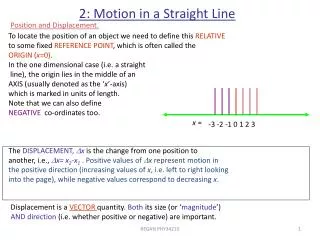
2- DISPLACEMENT; AVERAGE VELOCITY • Quantitative discussions of motion are based on measurements and calculations of positions, displacements, velocities, and accelerations. • We consider only translational motion, in which every part of an object moves in the same direction, and there is no rotation. Displacement: • The displacement of an object is not the same as the distance it has traveled. Example: Suppose you walk 10 m north, and then turn around and walk 10 m south. You have walked a total distance of 20 m. However, your displacement is the net change in your position, or zero in this case. • Displacement have a direction as well as a magnitude.
Average velocity: • The average velocity is defined in terms of the displacement, or the change in the position of an object that occurs in specified interval of time. Example: A car is moving north along a straight highway with marker posts every 100 m, and that it is observed to pass one of these posts every 5 s, as in Fig. 1a. During any one of these 5-s intervals, the displacement is 100 m, in 10-s interval, is 200 m; ... • The average velocity of a car during a specific time interval is the displacement divided by the time elapsed: • The average velocity is proportional to the displacement, and it has the same direction.
The average velocity can now be defined more symbolically using this notation. Suppose that at some time which we call t1 the car is observed to be at position x1 and that at a later time t2, it is located at x2. • The displacement is the difference in positions: ∆x = x2 – x1 The symbol ∆ is the Greek letter “delta”, and ∆x is read “delta x”. • The elapsed time between the observations is the difference: ∆t = t2 – t1 In this notation, the average velocity is the displacement divided by the elapsed time, • This definition is illustrated by the following example. (1.1)
Example 1.4: Using Eq. (1.1), find the average velocity of the car in Fig. 1.2 during the period from t = 10 to 25 s. Here t1 is 10 s and t2 is 25 s; from the graph, x1 = 200 m and x2 = 500 m. Thus
When an object undergoes uniform motion, its x-t graph is a straight line, as in the example of Fig. 1. • If the motion is accelerated, the graph is not a straight line, and the average velocity depends on the particular time interval chosen (see example 1.4). • Some times we can describe the motion of an object by an algebraic equation (see example 1.5: x=50m–(4.9m.s-2)t2). • If you know the average velocity, you can use that information to discuss the motion. For example, if you know how fast your car is going, you can figure out how long it will take to drive a given distance, or how far you can go in a specified time.
3- INSTANTANEOUS VELOCITY • The instantaneous velocity ( that is mean, the velocity at a particular instant in time) is determined by computing the average velocity for an extremely small time interval. Example 1.9: The motion of the car shown in Fig. 1.3 corresponds to the algebraic formula x = b t2, where b=1 m s-2. Find its average velocity from 3 to 3.1 s, 3 to 3.01 s, and 3 to 3.001 s.
Solution 1.9: when t = 3 s, the position is x = b t2 = (1 m s-2)(3 s)2 = 9m; when t = 3.1 s, x = 9.61 m. Thus the average velocity from 3 to 3.1 s is At t = 3.01 s, the position is x = (1 m s-2)(3.01 s)2 = 9.0601 m, so average velocity from 3 to 3.01 s is: At t = 3.001 s, the position is x = (1 m s-2)(3.001 s)2 = 9.0601 m, so average velocity from 3 to 3.01 s is:
As the time interval t is made smaller and smaller, the average velocity steadily approaches 6 m s-1. Therefore, the instantaneous velocity v at t = 3 s is 6 m s-1. • Mathematically, the instantaneous velocity v is said to be limit of the average velocity as Dt approaches zero. The process of evaluating this limit is called differentiation; v is called derivative of x with respect to t and is written as: • Positive values of instantaneous velocity correspond to motion toward increasing x, or in the + x direction. If v is negative, the object is moving in the – x direction.
4- ACCELERATION • Like the position, the velocity can change with time. The average acceleration a from time t1 to t2, if the velocity changes by v = v2-v1, is defined by: Example 1.14: The velocity of a slowing car is given by the equation: v = (20 m s-1) – (3 m s-2) t Find the average acceleration from t = 1s to t = 3s.
Solution 1.14: The average acceleration is The instantaneous acceleration: - The instantaneous acceleration a is found in much the same way as the instantaneous velocity. - We compute the average acceleration for progressively shorter time intervals. Then the instantaneous acceleration is the limit obtained as t approaches zero:
5- FINDING THE MOTION OF AN OBJECT:Equations of motion with a constant acceleration • Often the acceleration can be calculated theoretically or measured experimentally. • If the initial position and velocity are known, their later values can then be found from the acceleration. • In the special case where the acceleration is constant, we can find the equations of motion. • The change in velocity equals the area under the a-t graph over the time interval chosen. • The displacement is equal to the area under the v-t graph over the time interval chosen.
Example 1.16: A car initially at rest at a traffic light accelerates at 2 m s-2 when the light turns green. After 4s. What are its velocity and position? Solution 1.16 Since we know the acceleration a, the elapsed time t, and the initial velocity v0=0, we can use Eqs. 1.5 and 1.8 to find the velocity and displacement. Thus v = v0 + at = 0 + (2m.s-2) (4s) = 8 m.s-1 x = v0t + (1/2)a(t)2 = 0 +(1/2)(2m.s-2)(4s)2=16 m After 4s the car has reached a velocity of 8m.s-1 and is 16m from the light. Note that we could also have found x from Eq. 1.7, using our result for v.
THE ACCELERATION OF GRAVITY AND FALLING OBJECTS: • Falling objects undergo an acceleration, which we attribute to gravity, the gravitational attraction of the earth. • If gravity is the only factor affecting the motion of an object falling near the earth’s surface, and air resistance is either absent or negligibly small. So long as the object’s distance from the surface of the earth is small compared to the earth’s radius, it is found that: 1- The gravitational acceleration is the same for all falling objects, no matter what their size or composition. 2- The gravitational acceleration is constant. It does not change as the object falls. • The acceleration of gravity near the surface of the earth is denoted by g; it is approximately equal to: g = 9.8 m s-2 • Small variations in g occur as result of changes in latitude, elevation, and the density of local geological features. • An object initially thrown upward also has this acceleration . Its velocity steadily decreases in magnitude until it becomes zero at the highest point reached.
Example 1.20: A ball is dropped from a window 84 m above the ground. a) When does the ball strike the ground? b) What is the velocity of the ball when it strikes the ground? Solution 1.20 Let us choose positive values of x in the upward direction. a) v0=0, a=-g, the ball strikes the ground when x = -84 m. This happens after a time interval t , which satisfies: x = (1/2)a(t)2 or (t)2 = 2 x /a thus t = 4.14 s b) Using Eq. 1.5 with t = 4.14 s and v0=0, v = a t = -40.6 m.s-1