Hardware Design and The Petri Net
220 likes | 425 Vues
Hardware Design and The Petri Net. Abhijit K. Deb SAM, LECS, IMIT, KTH Kista, Stockholm. Outline. Petri net and HW design Characteristics Simulation Example: A set of communicating FSM Verification Conclusion. Petri Net and HW Modeling.

Hardware Design and The Petri Net
E N D
Presentation Transcript
Hardware Design andThe Petri Net Abhijit K. Deb SAM, LECS, IMIT, KTH Kista, Stockholm
Outline • Petri net and HW design • Characteristics • Simulation • Example: A set of communicating FSM • Verification • Conclusion Abhijit K. Deb
Petri Net and HW Modeling • Petri net is a general formalism to represent discrete event systems • For HW design, Petri net has been used in many different ways: • synthesis • HW/SW partitioning • simulation & verification Abhijit K. Deb
Petri Net Characteristics • Parallelism or concurrency is modeled better in a Petri net • The composition of state machines is complex; composition of Petri nets is simple • Petri nets are asynchronous in nature, however when synchronization is needed, that is also easy to model • There is no inherent measure of time in a Petri net Abhijit K. Deb
Verilog VL2aSTG petrify STG Mapped Netlist Synthesis using Petri Net C1 C2 C3 C1 C2 C3 clock Abhijit K. Deb
Simulation • Often, systems are modeled as a set of communicating FSMs • Problem: • FSMs are good for modeling sequential behavior but modeling concurrency and memory is difficult • state explosion • data value Abhijit K. Deb
Forming the Petri Net • Each state of the communicating FSMs are represented by a place, called state-place. • All synchronization signals are represented by two places: • a high place • a low place • A token can not exist in both of the places and both places can not be empty as well • Arcs are drawn between input places to transitions and transitions to output places • Reset signal gives the initial distribution of tokens in different places Abhijit K. Deb
S1 S2 FSM - PN wr sel cs sel=1, wr=1 / cs=1, rws=1 t1 cs – / cs=0, rws=0 S1 S2 rws t2 rws Petri Net Representation FSM Representation Abhijit K. Deb
Timing • Introduce clock-place to represent time • The clock-place is an input place for all transitions synchronous with that clock • Appearance of token in a clock-place represent the arrival of a clock edge and advances simulation time • For a system with multiple clocks, multiple clock-places are needed, where tokens appear according to the ratio of the speeds of the clocks involved Abhijit K. Deb
Handling Data • Storage (e.g., memory, register) and interconnect (e.g., bus) hold data • Data signals are viewed as placeholders • The placeholders can be of different type, an integer, array or a composite type like a record • They are updated with a transition firing either by an assignment operation or by a C-function call Abhijit K. Deb
Simulation Procedure 1. incidence matrix is formed for the Petri net derived from the FSM description of the system 2. reset signal gives the initial states of the signals and the communicating FSMs 3. clock place gets tokens to advance simulation time 4. using the present state of the net, enabled transitions are marked, that gives the firing vector 5. enabled transition(s) can be fired at any order 6. next state of the system is computed using the following: x’ = x + uA 7. based on the new state, if a given condition is true then update the placeholders for data values using an assignment operation or a C function call 8. repeat from step 3 as long as there are enabled transitions Abhijit K. Deb
Memory wrReq = 1 / Ack = 1 rdReq =1 / Ack =1 dtRdy = 1 / Ack =0 rdReq = 0 / Ack = 0 dtRdy =1 G4 M4 M1 C8 M3 C4 C6 C7 G3 C2 C1 G1 M2 G2 C3 C5 Ack =1 / dtRdy = 0 Gn Gn-1 1 Arbiter reqFrm1=1 / Grant1 =1 reqFrm1 =0 reqFrm1 =0 / Grant1 =0 reqFrm2=1 / Grant2 =1 reqFrm2 =0 reqFrm2=0 / Grant2 =0 … … A Network of FSM Core IO_rd =1 / reqFrm2=1 IO_wr =1 / reqFrm2 =1 Grant2 =1 / rdReq =1 Grant2 =1/ wrReq =1 Ack =1 / rdReq =0 Ack =1 / wrReq =0 dtRdy = 1 dtRdy = 1 / Ack = 1 Ack = 0 / dtRdy = 0 reqFrm2 =0 dtRdy =0 / Ack = 0 reqFrm2 =0 Abhijit K. Deb
A1 busRq M2 C2 C3 A2 C1 Petri net Representation IO_wr Memory Core arbiter M1 busRq wrRq t2 t4 t1 t5 t6 wrRq t3 grant grant Abhijit K. Deb
A1 busRq M2 C2 C3 A2 C1 Petri net Representation IO_wr Memory Core arbiter M1 busRq wrRq t2 t4 t1 t5 t6 wrRq t3 grant grant Abhijit K. Deb
A1 busRq M2 C2 C3 A2 C1 Petri net Representation IO_wr Memory Core arbiter M1 busRq wrRq t2 t4 t1 t5 t6 wrRq t3 grant grant Abhijit K. Deb
A1 busRq M2 C2 C3 A2 C1 Petri net Representation IO_wr Memory Core arbiter M1 busRq wrRq t2 t4 t1 t5 t6 wrRq t3 grant grant Abhijit K. Deb
A1 busRq M2 C2 C3 A2 C1 Petri net Representation IO_wr Memory Core arbiter M1 busRq wrRq t2 t4 t1 t5 t6 wrRq t3 grant grant Abhijit K. Deb
A1 busRq M2 C2 C3 A2 C1 Petri net Representation IO_wr Memory Core arbiter M1 busRq wrRq t2 t4 t1 t5 t6 wrRq t3 grant grant Abhijit K. Deb
A1 busRq M2 C2 C3 A2 C1 Petri net Representation IO_wr Memory Core arbiter M1 busRq wrRq t2 t4 t1 t5 t6 wrRq t3 grant grant Abhijit K. Deb
Specification Verification • Conservation: One token must exist in one of the high or low place of a signal, both of them can not be empty simultaneously. • Boundedness: Tokens can not grow in one of the places. • Safety property: the system will not get into a specific undesirable configuration, e.g., a deadlock or the emission of undesired output. • Liveness property: Some desired configuration will be visited eventually or infinitely often (fairness). Abhijit K. Deb
Conclusion • Systems can be simulated using Petri nets • The Petri net representation is bounded • The number of places is the summation of all the states plus twice the number of all the synchronization signals • Provides the necessary glue between different parts of the system, which is needed to perform a system simulation • The simulation shows dynamic behavior of the system • It is possible to perform certain specification verification using Petri net Abhijit K. Deb