Denoising by Wavelets

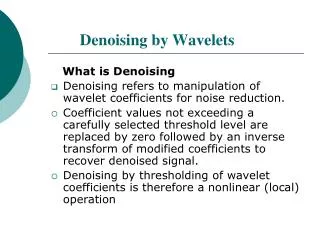
1. Denoising by Wavelets What is Denoising • Denoising refers to manipulation of wavelet coefficients for noise reduction. • Coefficient values not exceeding a carefully selected threshold level are replaced by zero followed by an inverse transform of modified coefficients to recover denoised signal. • Denoising by thresholding of wavelet coefficients is therefore a nonlinear (local) operation

2. Noise Reduction by Wavelets and in Fourier Domains • Comments • Denoising is a unique feature of signal decomposition by wavelets • It is different from noise reduction as used in spectral manipulation and filtering. • Denoising utilizes manipulation of wavelet coefficients that are reflective of time/space behavior of a given signal. • Denoising is an important step in signal processing. It is used as one of the steps in lossy data compression and numerous noise reduction schemes in wavelet analysis.

3. Denoising by Wavelets • For denoising we use thresholding approach applied on wavelet coefficients. • This is to be done by a judiciously chosen thresholding levels. • Ideally each coefficients may need a unique threshold level attributed to its noise content • In the absence of information about true signal, this is not only feasible but not necessary since coefficients are somewhat correlated both at inter and intra decomposition levels ( secondary features of wavelet transform).

4. True Signal Recovery • Thresholding modifies empirical coefficients (coefficients belonging to the measured noisy signal) in an attempt to reconstruct a replica of the true signal. • Reconstruction of the signal is aimed to achieve a ‘best’ estimate of the true (noise-free) signal. • ‘Best estimate’ is defined in accordance with a particular criteria chosen for threshold selection.

5. Thresholding • Mathematically, thresholding of the coefficients can be described by a transformation of the wavelet coefficients • Transform matrix is a diagonal matrix with elements 0 or 1. Zero elements forces the corresponding coefficient below or equal to a given threshold to be set to zero while others corresponding to one, retains coefficients as unchanged. • =diag(1, 2,….. N) with i={0,1}, i=1,…N.

6. Hard or Soft Thresholding. • Hard Thresholding. Only wavelet coefficients with absolute values below or at the threshold level are affected, they are replaced by zero and others are kept unchanged. • Soft Thresholding. Coefficiens above threshold level are also modified where they are reduced by the threshold size. Donoho refers to soft threshoding as ‘shrinkage’ since it can be proven that reduction in coef-ficient amplitudes by soft thresholding, also results in a reduction of the signal level thus a ‘ shrinkage’.

7. Hard and Soft Thresholding • Mathematically hard and soft thresholding is described as • Hard threshold: wm= w if |w|≥th, wm= 0 if |w|<th • Soft threshold : wm = sign(w)(|w|-th), |w|≥th, wm=0 , |w|<th

8. Global and Local Thresholding • Thresholding can be done globally or locally i.e. • single threshold level is applied across all scales, • or it can be scale-dependent where each scale is treated separately. • It can also be ‘zonal’ in which the given function is divided into several segments (zones) and at each segment different threshold level is applied.

9. Additive Noise Model and Nonparametric Estimation Problem • Additive Noise Model. Additive noise model is superimposed on the data as follows. f(t) = s(t) + n(t) n(t) is a random variable assumed to be white Gaussian N(0, σ). S(t) is a signal not necessarily a R.V. • Original signal can be described by the given basis function in which coefficients of expansion are unknown se(t)=∑αi φi (t) • Se(t) is the estimate of the true signal s(t). Note the estimate s^(t) is described by set of spanning function φi(t), chosen to minimize the L2 error function of the approximation ||s(t)-se (t)||2 . • As such denoising is considered as a non-parametric estimation problem.

10. Properties of Wavelets Utilized in Denoising • Sparse Representation. • Wavelet expansion of class of functions that exhibit sufficient degree of regularity and smoothness, results in pattern of coefficient behavior that can often be categorized into two classes: • 1) a few large amplitude coefficients and • 2) large number of small coefficients. This property allows compaction for compression and efficient feature extraction.

11. Wavelet Properties and Denoising • Decorrelation. Wavelets are referred to as decorrelators in reference to a property in which wavelet expansion of a given signal results in coefficients that often exhibit a lower degree of correlation among the coefficients as compared with that of the signal components. • Orthogonality. Intuitively, under a given standard DWT of a signal, this can be explained by the orthogonality of expansion and corresponding bases functions.

12. i.i.d. assumption • Under certain assumptions, coefficient in highest frequency band, can be considered to be statistically identically independent of each other

13. Examples of Signal Compaction and Decorrelation at Coefficient Domain

14. Signal Decorrelation at Coefficient Domain

15. Why Decorrelation by Wavelets • Coefficients carry signal information in subspaces that are spanned by basis functions of the given subspace. • Such bases can be orthogonal ( uncorrelated) to each other, therefore coefficients tend to be uncorrelated to each other • Segmentation of signal by wavelets introduce decorrealtion at coefficient domain

16. White Noise and Wavelet Expansion • No wavelet function can model noise components of a given signa ( no match in waveform for white noise). • White noise have spectral distribution which spreads across all frequencies. There is no match ( correlation) between a given wavelet and white noise • As such an expansion of noise component of the signal, results in small wavelet coefficients that are distributed across all the details.

17. Search fro Noise in Small Coeffs • S(t) = x(t) +n(t) An expansion of white noise component of the signal, results in small wavelet coefficients that are distributed across all the details. We search for n(t) of white noise at small coefficients in DWT that often residing in details

18. White Noise and High Frequency Details • At high frequency band d1, the number of coefficients is largest under DWT or other similar decomposition architectures. • As such, a large portion of energy of the noise components of a signal, resides on the coefficients of high frequency details d1 • At high frequency band d1, are short length basis functions and there is high decorrelation at this level( white noise)

19. White Noise Model and Statistically i.i.d. Coeffs • Decorrelation property of the wavelet transform at the coefficient level, can be examined in terms of statistical property of wavelet coefficients. • At one extreme end, coefficients may be approximated as a realization of a stochastic process characterized as a purely random process with i.i.d (identically independently distributed) random variable. • Under this assumption, every coefficient is considered statistically independent of the neighboring coefficients both atthe inter-scale (same sale) and intra-scale (across the scales) level.

20. White Noise Model and Multiblock denoising • However, in practice, often there exist certain degree of interdependence among the coefficients, and we need to consider correlated coefficients for noise models( such as Markov models). • In other models used to estimate noise, blocks of coefficients instead of single coefficients, are used as statistically independent • In Matlab, multi-block denoising at each level is considered

21. Main Task • Main task in denoising by wavelets: • Identification of underlying statistical distribution of the coefficients attributed to noise. • For signal, no structural assumption is made since in general it is assumed to be unknown. However, if we have additional information on the signal, we can use them and improve our estimation results

22. Main Task • Denoising problem is treated as an statistical estimation problem. • The task is followed by the evaluation of variance and STD of statistics of the noise model that are used as metrics for thresholding. • A’priori distributions may be imposed on the coefficients using Bay’s estimation approach after which denoising is treated asaparametric estimation problem

23. Alternative Models for Noise Reduction. • Basic Considerations • Additive Noise Model. Basic modeling structure utilizes additive noise model as stated earlier. x(i)=s(i)+ n(i) , i=1,2, … N • N is signal length, x(i) are the measurements, s(i) is the true signal value(unknown) and n(i) are the noise components(unknown) • n(i) is assumed to be white Gaussian with zero mean N(0,1). Standard deviation is to be estimated

24. Additive Noise Model and Linearity of Wavelet Transform • Under an orthogonal decomposition and additive noise model, linearity of wavelet transform insures that the statistical distribution of the measurements and white noise remain unchanged in the coefficient domain. • Under an orthogonal decomposition, each coefficient is decomposed into component attributed to the true signal values s(n) and to signal noise component n(k) as follows. cj= uj+dj i=1,2, .. n

25. Orthogonal vs Biorthogonal • In vector form C=U+D • C, U and D are vector representation of empirical wavelet coefficients, true coefficient values( unknown) and noise content of the coefficients respectively. • Note ‘additive noise model’ at the coefficient level while preserving statistical property of the signal and noise at the coefficient as stated above, is valid under orthogonal transformation where Parseval relationship holds. • It is not valid under biorthogonal transform. Under biorthogonal transform, white noise at the signal level will exhibit itself as colored noise since the coefficients here are no longer i.i.d but they are correlated to each other.

26. Principle Considerations 1. Assumption of Zero Mean Gaussian. • Under additive noise model and assumption of i.i.d. for the wavelet coefficients, we consider zero mean Gaussian distribution at the coefficient domain. • Mean centering of data can always be done to insure zero mean Gaussian assumption as used above.

27. Main Considerations • Preservation of Smoothness. • It can be proved thatunder soft thresholding, smoothness property of the original signal remains unchanged with high probability under variety of smoothness measures ( such as Holden or Sobolov smoothness measures). • Smoothness may be defined in terms of integral of squared mth derivative of a given function to be of finite value • This property and structural correlation of wavelet coefficients at consecutive scales, are used in wavelet-based zero-tree compression algorithm

28. Main Considerations • Shrinkage. Under soft thres-holding ( nonlinear operation at the coefficient level), it can be shown that • | xid |≤|xi| where xid is denoised signal component i.e. • denoising results in reduction of all the coefficients and shrinkage at the signal level as well.

29. Denoising Problem • Denoising problem is mainly estimation of STD and Threshold Level • Basic problem in noise reduction under Gaussian white noise, is centered around the estimation of standard deviation of the Gaussian noise  • It is then used to determine a suitable threshold

30. Alternative Considerations. • White Noise Model-Global (Universal) Thresholding. • Assume coefficients at the highest frequency details gives a good estimate of the noise content . • A white noise model is superimposed on the coefficients at the highest frequency detail level d1 • An estimate of the standard deviation at the d1 level is then used to arrive at a suitable threshold level for coefficient thresholding at all levels. • This approach is a global thresholding which is applied to all detail coefficients

31. Level Dependent Thresholds • Nonwhite (Colored) Noise Model. • Under this model, still white noise model is imposed on the coefficients of details, however threshold levels are considered to be level(scale) dependent. • Gaussian white noise model is imposed on detail coefficients using standard deviation and threshold level at each level separately.

32. Comments on Estimation Problem, Near Optimality under other Optimality Criteria • Wavelet denoising (WaveShrink) utilizes a nonparametric function estimation approach for noise thresholding. • It has been shown that statistically, denoising is considered to be: asymptotically near optimal over a wide range of optimality criteria and for large class of functions found in scientific and engineering applications( see ref by Donoho).

33. Inaccuracy of Assuming Gaussian Distribution N(1,0), Result Evaluations • Assumption of Gaussian distribution at d1 level may not always be valid • Distribution of the coefficient at d1 often exhibit a long tail as compared with standard Gaussian(peaky distribution) This can also be observed in the case of sparsely distributed large amplitude coefficients or outliers. • Under such condition, application of global thresholding may be revised and results of the thresholding be examined in light of actual data analysis and performance of denoising.

34. Inaccuracy of Assuming Gaussian Distribution • Fig.2 Peaky Gaussian-like pdf of the coefficients with long tail ends

35. Signal Estimation and Threshold Selection Rules • Use statistical estimation theory applied on probability distribution of the wavelet coefficients • Use criteria for estimation of statistical parameters and selecting threshold levels • A loss function which is referred to as ‘risk function’ is defined first. • For Loss function we often use L2 norm of the errori.e. variance of estimation error, i.e. difference between the estimated value and actual unknown value

36. Risk (Loss Function) • We use expected value of the error as loss function since we are dealing with noisy signal which is a random variable and is therefore described in term of expected value. • Minimization of risk function results in an estimate of the variance of the coefficient.

37. Risk (Loss) Function • X is the actual (true) value of the signal to be estimated ( or coefficients) and X’ is an estimate of the signal X ( or coefficients ). • Since noise component is assumed to be zero mean Gaussian, the difference is a measure of an error based on the additive noise model and given risk function. • It is a measure of the energy of the noise i.e.∑[n(k)]2 • Thus optimization procedure as defined above, attempts to reduce the energy of the signal X by an amount equal to the energy of the noise and thus compensating for the noise in the sense of L2 norms.

38. Minimization of the risk function at coefficient level • Under an orthogonal decomposition, minimization of risk function at the signal level, can equivalently be defined at the coefficient level. • R(X^ ,X)= E||X^- X||2=E||W-1(C^ -C)||2 =E||(C^ -C)||2 • C^ is the estimate of the true coefficient values. We have used additive noise model and wavelet transform in matrix form C=WX as described below. X=S + σn, C=WX, X=W-1 C • Accordingly, minimization of the risk function at the coefficient level results equivalently in estimating the true value of the signal.

39. Use of Minimax Rule • One ‘best’ estimate is obtained using minimax rule indicated below: • Minmax R(X^,X)= inf sup R(X^,X) • Under minmax rule, worst case condition is considered, i.e. Sup R(X^,X) Here our objective is to mimimize the risk under worst case condition (i.e. obtain Min Max R) .

40. Global/Universal Thresholding Rule • Under the assumption of i.i.d. for the wavelet coefficients and Gaussian white noise, one can show that • Under soft thresholding, the actual risk is within log(n) factor of the ideal risk where the error is minimal (on the average). • This results in the following threshold value referred to as Universal Thresholding which minimizes max risk as defined above. Th=(2 log n), =MAD/.6745 MAD is ‘median absolute deviation’ of the coefficients median({|d J−1,k|: k = 0, 1, . . . , 2^(J−1) −1}) Ref: Donoho D.L. ”Denoising by Soft thresholding”, IEEE Trans on Information Theory, Vol 41,No.3 May 1995,pp 613-627

41. Universal Thresholding Rule • Underlying basis for above threshold rule is based on the assumption of i.i.d for set of random variables X1, . . . , Xn having a distribution N(0, 1). • Under this assumption, we can say the following for the probability of maximum absolute value of the coefficients. P{max |Xi|, 1≤i≤n> √ 2 logn}→ 0, as n → ∞ Note Xi refers to noise

42. Universal Thresholding Rule • Therefore, under universal thresholding applied to wavelet coefficients, we can say the following. with high probability every sample in the wavelet transform (i.e.coefficient) in which the underlying function is exactly zero will be estimated as zero

43. Universal Thresholding Rule in WP • Universal threshold estimation rule when applied to wavelet packet is to be adjusted to the length of decomposition which is nlog(n). Threshold is then Th=[2 log(nlog(n)].

44. Level Dependent Thresholding • In level dependent thresholding, thresholds are rescaled at each level to arrive at a new estimate corresponding to the standard deviation of wavelet coefficients at that level. • We consider white noise model and Gaussian distribution for the coefficient at each level. • This is referred to ‘mln’ [multilevel noise model] in Matlab toolbox. Threshold level is determined as follows. Th(j,n) = σj(2 log nj), σj =MADj /.6745

45. Stein Unbiased Risk Estimator( SURE) • A criteria referred to as Stein Unbiased Risk Estimator abbreviated by SureSrink, utilizes statistical estimation theory in which an unbiased estimate of loss function is derived • Suppose X1, . . . , Xs are independent N(μi, 1),i = 1, . . . , s, random variables. The problem is to estimate: mean vector μ = (μ1, . , μs)with minimum L 2-risk. • Stein states that the L2-loss can be estimated unbiasedly using any estimator μ that can be written as μ(X) = X + g(X), where the function g = (g1, . . . , gs)is weakly differentiable.

46. SURE Estimator • Under SURE criteria, following is considered as an estimate of the loss function. E||(x)- e||^2 =E SURE(th:x) where SURE(th;x)=s-2#B{i:|Xi|≤ th}+ (min(|xi|,th)^2 where (x) is a fixed estimate of the mean of the coefficients and #B denotes the cardinality of a set B. • It can be shown that SURE(th;x) is an unbiased estimate of the L2-risk, i.e. µ|| µλ(X)- µ||^2 = µSURE(th; X). • Threshold level λ is based on minimum value of SURE loss function which is defined as Ths = arg min th Sure(th;x)

47. Other Thresholding Rules • Fixed Form thresholding is the same as Universal Thresholding Th=(2 log n), =MAD/.6745 • Minimax refers to finding the minimum of the maximum mean square error obtained for the worst function in a given set

48. Rigorous SURE Denoising • Rigorous SURE (Stein’s Unbiased Risk Estimate), a threshold-based method with a threshold where n is the number of samples in the signal(i.e. coefficients)

49. Heuristic SURE • Heuristic SURE is a combination of Fixed Form and Rigorous SURE • ( for details refer to Matlab Helpdesk)

50. Results of Denoising Application on CDMA Signal • At SNR = 3 dB, MSE between the original signal and the noisy signal is 0.99. • The following table shows MSE after denoising: Wavelet Haar,Bior3.1,Db10,Coif5, • fixed form, white noise 0.55 0.64 0.46 0.46 • RigSURE, white noise 0.36 0.41 0.27 0.27 • HeurSURE,wh. Noise 0.42 0.41 0.27 0.28, • Minimax, white noise 0.46 0.46 0.34 0.33, • Minimax, nonwhite 0.53 1.09 0.44 0.32,