AI Pathfinding
AI Pathfinding. Representing the Search Space To perform pathfinding , an agent or the pathfinding system needs to understand the level. A n agent only needs a representation of the level that takes into account the most important and relevant information.

AI Pathfinding
E N D
Presentation Transcript
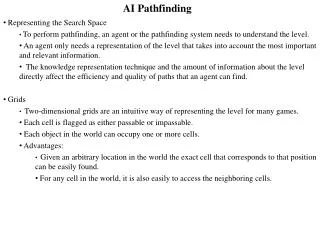
AI Pathfinding Representing the Search Space To perform pathfinding, an agent or the pathfinding system needs to understand the level. An agent only needs a representation of the level that takes into account the most important and relevant information. The knowledge representation technique and the amount of information about the level directly affect the efficiency and quality of paths that an agent can find. Grids Two-dimensional grids are an intuitive way of representing the level for many games. Each cell is flagged as either passable or impassable. Each object in the world can occupy one or more cells. Advantages: Given an arbitrary location in the world the exact cell that corresponds to that position can be easily found. For any cell in the world, it is also easily to access the neighboring cells.
AI Pathfinding Representing the Search Space Waypoint graphs A waypoint graph specifies the lines in the level that are safe for traversing. An agent can choose to walk along any of these lines without having to worry about running into major obstacles or falling into ditches or off a ramp. The waypoint nodes are connected through links. A link connects exactly two nodes together, indicating that an agent can move safely between the two nodes by following along the link. The nodes of a waypoint graph can store additional information such as a radius. The radius can be used to associate a width with the links so that the agents do not have to follow the links very closely. One of the biggest advantages of waypoint graphs is that they can easily represent arbitrary three-dimensional levels.
AI Pathfinding Representing the Search Space Navigation meshes They bring the best of both grids and waypoint graphs together. Every node of a navigation mesh represents a convex polygon or area, as opposed to a single point. Any two points inside a convex polygon can be connected without crossing an edge of the polygon. An agent can safely move to any other point inside the polygon without leaving the polygon. An edge of the polygon is shared with another polygon, indicating that the two nodes are linked. An edge of the polygon is not shared with any other polygon, indicating that the edge should not be crossed. Edges that are not shared with other nodes can be used to stop the bots from running into obstacles or falling off a cliff. Nodes store triangles vs. an n-sided convex polygons. Navigation meshes tie pathfinding and collision detection together.
AI Pathfinding Pathfinding A path is a list of cells, points, or nodes that an agent has to traverse to get from a start position to a goal position. In general, a large number of different paths can be taken to reach the same goal. Complete pathfinding algorithms: guarantee to find a path Optimal pathfinding algorithms: guarantee to always find the most optimal path Random-trace Allow the agent to move toward the goal until it reaches the goal or runs into an obstacle. If it runs into an obstacle, it can randomly choose to trace around the object in a clockwise or counterclockwise manner. It can then trace around the object until it can head toward the goal without immediately running into an obstacle. The agent can repeat this procedure until the goal is reached. The weakness of this algorithm if the map has concave or even large convex obstacles One of the fundamental problems with this algorithm is that it is incapable of considering a wide variety of paths.
AI Pathfinding Pathfinding Understanding the A* algorithm Consider a wide variety of paths. Keep track of numerous paths simultaneously Consider every possible part of the map to find a path to the goal. Keeping track of the paths. A path can be described as an ordered list of subdestinations. PlannerNode stores the position of a cell and a pointer to another PlannerNode that specifies which of the neighboring cells has led us to the cell. By chaining these nodes together using the parent pointers, a path between a starting cell and a goal cell can be represented. By creating additional paths that extend existing paths, an algorithm can work its way through the map in search of the goal. Open (node) list: keeps track of paths that still need to be processed. When a path is processed, Closed (node) list: keep those nodes that do not correspond to the goal cell and have been processed already.
AI Pathfinding Pathfinding Understanding the A* algorithm The node that reaches the goal is part of the path between the start and the goal. Once the goal has been reached, the path between start and goal can be obtained by traversing the parent pointer of the PlannerNodes starting from the node that reached the goal and ending with the root node. Guarantee to find a solution if one exists, regardless of how complicated the map The algorithms make sure there is no more than one node for any given cell of the grid, Before creating a successor node.
AI Pathfinding Pathfinding Breadth-first Breadth-First tries to find a path from the start to the goal by examining the search space ply-by-ply. (exhaustive search) It checks all the cells that are one step (or ply) from the start, and then checks cells that are two plies from the start, and so on. The algorithm always processes the node that has been waiting the longest, using a queue as the open list. Shortcoming: It consumes a lot of memory and CPU cycles to find the goal. It does not take advantage of the location of the goal to focus the search effort. It searches just as hard in the direction away from the goal as it does toward the goal. Result: It finds the most optimal solution in terms of (number of ) plies on the result path..
AI Pathfinding Pathfinding Best-first It uses problem-specific knowledge to speed up the search process. (heuristic search) It tries to head right for the goal. It computes the distance of every node to the goal and use a priority queue as the open list that is sorted by the heuristic cost. Through every iteration of the loop, the node that is closest to the goal is processed. On average, Best-First is much faster than Breadth-First and uses significantly less memory. It typically creates very few nodes and tends to find “good quality” paths. Shortcoming: It can end up heading in a direction that does not necessarily result in finding an optimal path. The distance-to-goal measure is a heuristic or rule- of-thumb that can pay off quite often. However, it is not always the right thing to do. Best-First is still a complete algorithm
AI Pathfinding Pathfinding Dijstra Similar to Breadth-First but always finds the optimal solution. Dijkstra keeps track of the cost of the path from start to any given cell. It always processes the cheapest path in the open list. Thismeans that every PlannerNode needs to store the accumulated cost that was paid to get to it from the start node. When Dijkstra generates a successor node, it adds the cost of the current node to the cost of going from the current node to the successor node. If the move from the current node to the successor node is a diagonal move, some additional cost should be added since a longer distance is traveled. If a node has been created already for a cell of the map, it still checks of the new path is better than the old one. No other algorithms can find paths more optimal than the ones found by Dijkstra. Dijkstra is an exhaustive search and therefore consumes a lot of memory and CPU cycles to find a path.
AI Pathfinding Pathfinding A* A* resolves most of the issues with Breadth-First, Best-First, and Dijkstra. It tends to use significantly less memory and CPU cycles than Breadth-First and Dijkstra. It can guarantee to find an optimal solution as long as it uses an admissible heuristic function (a function that never overestimates the true cost). A* combines Best-First and Dijkstra by taking into account both the given cost (the actual cost paid to reach a node from the start) and the heuristic cost (the estimated cost to reach the goal). A* keeps the open list sorted by final cost: Final Cost = Given Cost + (Heuristic Cost * Heuristic Weight) Heuristic weight can be used to control the amount of emphasis on the heuristic cost versus the given cost. The weight can be used to control whether A* should behave more like Best-First or more like Dijkstra. To guarantee that A* finds the optimal solution, the heuristic function used to compute the heuristic cost should never overestimate the actual cost of reaching the goal. By nature, the distance formula is a non-overestimating heuristic function for pathfinding.