Download

1 / 57
570 likes | 791 Vues
The Corporation Investment, mergers, and growth. Chapter 7 Investment. Overview. Investment in Macro- and Microeconomics What should be considered as Investment? Capital expenditures R&D Mergers Determinants Theories Tests MM Theorems CAPM Returns on Investment

E N D
The CorporationInvestment, mergers, and growth Chapter 7 Investment
Overview • Investment in Macro- and Microeconomics • What should be considered as Investment? • Capital expenditures • R&D • Mergers • Determinants • Theories • Tests • MM Theorems • CAPM • Returns on Investment • Methods using Accounting Data • Methods using Stock Market Data
7.2 The Accelerator Theory • focuses only on the marginal returns side of the investment scissors. • Let f(K,L) be a linear homogeneous production function, and i and w be constant. • The firm’s output expansion path is then a straight line, with its output being a constant proportion of its capital stock, Q = (1/b)K (7.3) • If demand conditions are such that its optimal output in time t is Qt, then its desired capital stock in period t can be written as KDt = bQt (7.4)
The purchase and installation of capital equipment takes time, and thus it is reasonable to assume that a firm can adjust its capital stock only a partial way towards its desired level. • If a represents this adjustment factor, 0 < a < 1, then the change in capital stock in any period (investment) is proportional to the difference between existing and desired capital stock. It = Kt − Kt−1 = a(KDt − Kt−1) (7.5) • Using equation (7.4) to replace the desired capital we obtain the basic accelerator equation.
It = abQt − aKt−1 (7.6) Demand Supply for Capital Stock
7.3 Cash Flow Models • The Basic Hypothesis • managers have a desired flow of investment rather than a desired capital stock. It − It−1 = a(IDt − It−1) (7.7) where a is an adjustment factor (0<a<1) • The desired flow of investment in period t is proportional to some measure of cash flow, Ft. IDt = bFt (7.8) • Substituting (7.8) into (7.7) yields the basic cash flow investment equation It = abFt + (1 − a)It−1 (7.9) • Today’s investment is a function of cash flow and lagged investment.
When estimating equation (7.9) two measures of cash flow have generally been used • profits plus depreciation, or • profits plus depreciation less dividends. • Use of the second measure implicitly assumes that dividends are a higher priority use of cash flow than investment and are thus decided first. This assumption in turn raises the question of what determines dividends. We shall return to this issue later in the chapter. • Difference to the accelerator model: • the simple accelerator model stresses only the demand for capital side of the investment decision, • the simple cash flow model stresses only the cost of capital side. • The difference between the two is depicted with the help of Figure 7.2.
It is apparent that cash flow can be an important determinant of investment, if the firm’s cost of capital rises significantly when it has to resort to external sources for funds. • We discuss three explanations that have been given for why such a rise in the cost of capital might be expected as the firm enters the external capital market. • Transaction Costs • Asymmetric Information • Managerial Discretion
(1) Transaction Costs (Duesenberry, 1958) • External capital is more costly than internal capital because of the transaction costs of raising capital externally. • Bonds or common shares must be printed, • Investment bank fees must be paid, • Advertisements must be placed in newspapers, etc. • The next table shows that issuing securities may be prohibitively costly for small firms. • Issue costs for debt securities are lower than for equity--the costs for a large debt issue are less than 1 percent--but show the same economies of scale. • Debt issues are cheaper because administrative costs are somewhat less and because underwriters require compensation for the greater risks they take in buying and reselling stock.
Issue costs as a percent of proceeds for registered issues of common stock during 1971-1975 Source: C. W. Smith, "Alternative Methods for Raising Capital: Rights versus Underwritten Offerings,“ Journal of Financial Economics, 5:273-307 (December 1977).
Hierarchy of Finance Cost of internal capital < Cost of debt < Cost of equity
(2) Asymmetric Information(Myers and Majluf, 1984) • Basic Assumptions of the Model • There is a profitable investment opportunity, however the firm has not enough internal cash flows to finance it. • The firm’s debt capacity has been reached. • Managers know the true value of a company’s existing assets and investment opportunities and the capital market does not. • Basic Results • The capital market can undervalue the company’s shares. • If managers maximize the wealth of their existing (old) shareholders, then they might forgo a profitable investment opportunity.
How the Model Works • There are two possible states of the world with an equal probability of occurring. The firm’s managers are contemplating an investment of 100 with the net returns in both states given below:
At this time, the market is uncertain as to whether state 1 or state 2 will occur. • The value of the shares of the existing shareholders at this time should the managers undertake the investment is P’ = 0.5 ( 150 + 20 ) + 0.5 ( 50 + 10 ) = 115 • The value of the shares of the new shareholders, E = 100. • Thus, the old shareholder’s shares will be worth P’ / (P’ + E) fraction of the value the firm is eventually worth once the market learns the true state of the world is. • The new shareholder’s shares will be worth E / (P’ + E) fraction of the value the firm is eventually worth once the market learns the true state of the world is. • In state 1: VOLD1 = (115 / (115 + 100) ) * 270 = 144.41 VNEW1 = (100 / (115 + 100) ) * 270 = 125.58 • In state 2: VOLD2 = (115 / (115 + 100) ) * 160 = 85.58 VNEW2 = (100 / (115 + 100) ) * 160 = 74.41
If managers know that State 1 will occur, they will not issue any shares and they will not be able to undertake the investment. To see this compare the value of the shares of the existing shareholders with and without investment (144.41 < 150 ). • If the firm had a 100 in cash flow, it could finance the investment without harming the existing shareholders. • This result has been used as a justification to include CF as an explanatory variable in investment equations.
(3) Managerial Discretion • Marris’ growth model: • managers wish to expand the growth rate of their company beyond the level which maximizes shareholder wealth, • while maintaining the company’s share price at a sufficiently high level to avoid a takeover by outsiders who will dismiss the managers. • The managers’ utility function can thus be written as a function of the growth rate of the firm, g, and the probability of its being taken over, p U = U(g, p), with ∂U/∂g > 0, and ∂U/∂p < 0 • The probability of takeover increases as the share price falls.
The market value of the firm’s equity is the present discounted value of its dividend payments • Et: the market value of outstanding equity, • PSt: the price of a common share • NSt: the number of shares outstanding, • Divt+j: the dividends payment in year t+j, • i : the firm’s cost of capital. • Thus, share price rises ceteris paribus with dividends. • If we assume that all cash flows go either to dividends or investment, Ft ≡ It+Divt, then the firm’s share price falls as investment increases, and the probability of takeover rises as investment increases, p = p(I), p‘(I) > 0.
A growth-seeking management invests more than the amount that maximizes shareholder wealth, and thus for it the marginal impact of investment on share price is negative. • The marginal impact of investment on growth is positive, g‘(I) > 0. A growth-oriented management’s utility-maximizing level of investment thus satisfies the following condition
7.5 Expectations Theories of Investment • The accelerator and neoclassical theories both make today’s investment a function of today’s output. A firm invests not to produce today’s output, however, but tomorrow’s. • Yehuda Grunfeld (1960) proposed that investment should depend on a variable that captures expected future growth in the demand for capital. • He proposed the firm’s current market value, a variable that varies across firms both because of scale differences, and because of differences in market expectations regarding future growth rates. • Thus the Grunfeld model might be written as one in which KD = bM
The q-theory of investment incorporates the basic assumptions and conditions of the neoclassical model. • Under these assumptions, differences in q across firms reflect differences in desired capital stocks relative to actual capital stocks and thus should explain differences in investment, without actually having to measure the costs of capital of individual firms. • Both the q-theory of investment and the neoclassical theory make rather strong assumptions about the functioning of the capital market, and its effects on investment decisions. • These assumptions can be justified by appeal to modern finance theory. • Given the importance of this theory to the investment decision, we shall take a brief detour in the following two sections to examine some of the basic propositions of this theory.
7.6 The Neoclassical Cost of Capital and theModigliani and Miller Theorems 1) The Irrelevance of Debt and Dividends • If managers maximize the wealth of their shareholders, then they should invest only in positive NPV projects, i.e., those that offer a return (r) greater than the cost of capital (i), or r/i>1. • Franco Modigliani and Merton Miller (1958, 1961) showed that this opportunity cost (i) is the appropriate measure of the firm’s cost of capital, regardless of whether the firm uses internal funds, or new debt, or new equity to finance investment. • We assume that companies with similar risks can be grouped into risk classes.
Definitions: • j = risk class • Π = earnings per share • P = price of common share • The cost of capital, ij, of a firm in the jth risk class is • Theorem 1. The cost of capital, ij, is independent of the firm’s capital structure. • Proof: • Ej: the value of the common stock of company j • Pj: share price • Nj: number of shares outstanding • Dj: total debt • r: the risk-free rate of return • V = E + D
We wish to show that • V = Total Profits / cost of capital, and • V is independent of the proportions of E and D. • Let U and L be two firms in the same risk class with the same level of total profits : Note that
Consider an investor wishes to earn a gross return of • There are two possible routes s/he can take to achieve it.
If VL <VU, action 2 is cheaper, all investors will choose it, PL will increase, PU will decrease until VL = VU . • If VL > VU, action 1 is cheaper, all investors will choose it, PL will decrease, PU will increase until VL = VU .
7.8 Empirical Investigations of the Determinants ofInvestment • Most empirical studies of investment estimate a single model or hypothesis about the determinants of investment, and usually conclude that the data are consistent with the hypothesized relationship. • All of the models of investment discussed in this chapter have found empirical support in the literature. • Much more rare are empirical studies that compare two or more hypotheses about the determinants of investment. One of the first, and most ambitious of these, was by Jorgenson and Siebert (1968). • They sought to compare the performance of the accelerator, cash flow, expectations and neoclassical models of investment. They did so by estimating equations that differed only in the definition of the desired capital stock, and the lag structure allowed. The assumptions made with respect to the desired capital stock were as follows:
Results: Neoclassical > Accelerator ≈ Expectations > CashFlow
Jorgenson and Siebert drew their conclusions from time-series estimates of investment equations for 15 large U.S. companies. • J. Walter Elliott (1973) reestimated the four Jorgenson/Siebert models both cross-sectionally and with time series, and expanded the sample to 184 companies. • Elliott’s rankings of the models were
Grabowski and Mueller (1972) compared the performance of a neoclassical model against that of a cash flow model motivated by the managerial discretion growth hypothesis (hereafter MDH). • They specified equations for capital investment, R&D and dividends, and were the first to emphasize the importance of the dividends equation in testing the MDH against the neoclassical model. • G&M concluded that the MDH outperformed the neoclassical model based on • its overall fit to the data, • the particularly good fit of the dividends equation in the MDH, and • the strong performance of cash flow in both the investment and R&D equations of the MDH in comparison with the weak performance of both measures of the neoclassical cost of capital employed.
Owen Lamont (1997) • petroleum companies • a significant decrease in investment in non-petroleum activities following a sudden drop in their cash flows in 1986. • It appeares that the petroleum firms regard investment in non-petroleum operations as a discretionary investment which they only undertook when their cash flows were high.
Fazzari, Hubbard, and Peterson (1988) • first paper that tests the AIH • a sample of 422 US corporations was divided into low, medium and high retention ratio subsamples, • cash- flow / investment equations that also include Tobin’s q to capture differences in investment opportunities. • They estimate positive coefficients on cash flow for all three subsamples that increased in size as the level of retentions rose, and interprete this finding as supportive of the AIH.
Devereux and Schiantarelli (1990) • tried to identify both financial constraints and information asymmetries in their study of 720 UK corporations by dividing their sample by size, growth, and age. • Some support for the AIH was found. For example, cash flow had a (slightly) higher coefficient in the small, young firm subsample than in the small, old firm subsample, as one expects if the market learns to evaluate firm investment opportunities with time
Hoshi, Kashyap and Scharfstein (1991) • They divided their sample of 146 Japanese corporations into independent and group firms, with the former having dispersed outside ownership, and the latter being parts of groups of companies with much cross-holding of one another’s shares. • Hoshi et al. hypothesize that group firms are not subject to asymmetric information problems when financing their investments, because of the access to information other members have. • Consistent with this hypothesis, they find that cash flow has a positive and significant coefficient only in the investment equation for the independent companies. • Similar evidence has been provided for small firms in the United States (Petersen and Rajan, 1994), and for Italy (Schiantarelli and Sembenelli, 2000).
Because it takes some time before invested funds begin to produce profits, the regression equation must be properly lagged. To adjust for this, BHMQ experiment with a number of different lag structures consisting of 2, 3, 4, 5 and 7 years. BHMQ then break investment down into the three sources of finance: cash flow (P), new debt (D), and new equity (N) and consider these components as separate independent variables. Their coefficients are interpreted as the returns on the three sources of capital. Results:
Two important implications: (1) reconfirmation of the widely accepted pecking order hypothesis. (2) Since corporate investment has historically been financed largely through retained earnings, the extremely low return to this source of finance raises the possibility that marginal returns to investment may have been below the cost of capital during this period.
Fisher and Lorrie's (1964) estimates of returns on the market portfolio of common shares in 1950's range from 13 to 18 %