Download

1 / 23
230 likes | 665 Vues
Simulating Exchangeable Multivariate Archimedean Copulas and its Applications. Authors: Florence Wu Emiliano A. Valdez Michael Sherris. Literatures. Frees and Valdez (1999) “Understanding Relationships Using Copulas” Whelan, N. (2004) “Sampling from Archimedean Copulas”

E N D
Simulating Exchangeable Multivariate Archimedean Copulas and its Applications Authors: Florence Wu Emiliano A. Valdez Michael Sherris
Literatures • Frees and Valdez (1999) • “Understanding Relationships Using Copulas” • Whelan, N. (2004) • “Sampling from Archimedean Copulas” • Embrechts, P., Lindskog, and A. McNeil (2001) • “Modelling Dependence with Copulas and Applications to Risk Management”
This paper: • Extending Theorem 4.3.7 in Nelson (1999) to multi-dimensional copulas • Presenting an algorithm for generating Exchangeable Multivariate Archimedean Copulas based on the multi-dimensional version of theorem 4.3.7 • Demonstrating the application of the algorithm
Exchangeable Archimedean Copulas • One parameter Archimedean copulas • Archimedean copulas a well known and often used class characterised by a generator, φ(t) • Copula C is exchangeable if it is associative • C(u,v,w) = C(C(u,v),w) = C(u, C(v,w)) for all u,v,w in I.
Archimedean Copulas • Charateristics of the generator φ(t): • (1) = 0 • is monotonically decreasing; and • is convex (’ exists and ’ 0). If ’’ exists, then ’’ 0 • C(u1,…,un) = -1((u1) + … + (un))
Archimedean Copulas - Examples • Gumbel Copula • (t) = (-log(u))1/ • -1(t) = exp(-u) • Frank Copula • (t) = - log((e-t – 1)/(e- – 1) • -1(t) = - log(1 – (1 - e- )e-t) /log()
Theorem 4.3.7 Let (U1,U2) be a bivariate random vector with uniform marginals and joint distribution function defined by Archimedean copula C(u1,u2) = -1((u1) + (u2)) for some generator . Define the random variables S = (u1)/((u1) + (u2)) and T = C(u1,u2). The joint distribution function of (S,T) is characterized by H(s,t) = P(S s, T t) = s KC(t) where KC(t) = t – (t)/ ’(t).
Simulating Bivariate Copulas Algorithm for generating bivariate Archimedean copulas (refer Embrecht et al (2001): • Simulate two independent U(0,1) random variables, s and w. • Set t = KC-1(w) where KC(t) = t – (t)/ ’(t). • Set u1 = -1(s (t)) and u2 = -1((1-s) (t)). • x1 = F1-1(u1) and x2 = F2-1(u2) if inverses exist. (F1 and F2 are the marginals).
Theorem for Multi-dimensional Archimedean Copulas (1) Let (U1,…,Un)’ be an n-dimensional random vector with uniform marginals and joint distribution function defined by the Archimedean copula C(u1,…,un) = -1((u1) + … + (un)) or some generator . Define the n tranformed random variables S1,…,Sn-1 and T, where Sk = ((u1) + … + (uk)) / ((u1) + … + (uk+1)) T = C(u1,…un) = -1((u1) + … + (un))
Theorem for Multi-dimensional Archimedean Copulas (2) The joint density distribution for S1,…,Sn-1 and T can be defined as follows. h(s1,s2,…,sn,t) = |J| c(u1,…un) or h(s1,s2,…,sn-1,t) = s10s21s32…. sn-1n-2 -1(n)(t)[(t)] /’(t) Hence S1,…,Sn-1 and T are independent, and • S1and T are uniform; and • S2,…,Sn-1 each have support in (0,1).
Theorem for Multi-dimensional Archimedean Copulas (3) Distribution functions for Sk: Corollary: The density for Sk for k = 1,2,…n-1 is given by fSk(s) = ksk-1, for s (0,1) The distribution functions for Sk can be written as: FSk(s) = sk , for s (0,1) Corollary: The marginal density for T is given by: fT(t) = -1(n)(t)[(t)]n-1 ’(t) for t (0,1)
Algorithm for simulating multi-dimensional Archimedean Copulas • Simulate n independent U(0,1) random variables, w1,…wn. • For k = 1,2,…, n-1, set sk=wk1/k • Set t = FT-1(wn) • Set u1 = -1(s1…sn-1(t)), un = -1((1-sn-1) (t)) and for k = 2,…,n , uk = -1((1-sk-1)sj(t). • xk = Fk-1(uk) for k = 1,…,n.
Example: Multivariate Gumbel Copula • Gumbel Copulas • (u) = (-log(u))1/ • -1(u) = exp(-u) • -1(k) = (-1)k exp(-u)u-(k+1)/ k-1(u) • k (x) = [(x-1) + k] k-1 (x) - ’k-1 (x) • Recursive with 0 (x) = 1.
Normal vs Lognormal vs Gamma Example: Gumbel Copula (3)
Application:VaR and TailVaR (1) • Insurance portfolio • Contains multiple lines of business, with tail dependence • Copulas • Gumbel copula – distributions have heavy right tails • Frank copula – lower tail dependence than Gumbel at the same level of dependence • Economic Capital: VaR/TailVaR • VaR: the k-th percentile of the total loss • TailVaR: the conditional expectation of the total loss at a given level of VaR (or E(X| X VaR))
Density of Gumbel Copulas Density of Frank Copulas Application: VaR and TailVaR (2)
Application: VaR and TailVaR (3) • Assumptions: • Lines of business: 4 • Kendall’s tau = 0.5 (linear correlation = 0.7) • theta = 2 for Gumbel copula • theta = 5.75 for Frank copula • Mean and variance of marginals are the same
Frank Gumbel Application: VaR and TailVaR (4)
Application: VaR and TailVaR (5) • Gumbel copula has higher TailVaR’s than Frank copula for Lognormal and Gamma marginals • Lognormal has the highest TailVaR and VaR at both 95% and 99% confidence level.
Gumbel Frank Application: VaR and TailVaR (6)
Impact of the choice of Kendall’s correlation on VaR and TailVaR Application: VaR and TailVaR (7)
Conclusion • Derived an algorithm for simulating multidimensional Archimedean copula. • Applied the algorithm to assess risk measures for marginals and copulas often used in insurance risk models. • Copula and marginals have a significant effect on economic capital