Mathematical Modeling and Engineering Problem solving Chapter 1
Mathematical Modeling and Engineering Problem solving Chapter 1. Every part in this book requires some mathematical background. Computers are great tools, however, without fundamental understanding of engineering problems, they will be useless.

Mathematical Modeling and Engineering Problem solving Chapter 1
E N D
Presentation Transcript
Mathematical Modeling and Engineering Problem solvingChapter 1
Every part in this book requires some mathematical background
Computers are great tools, however, without fundamental understanding of engineering problems, they will be useless.
Finite element analysis (FEA) and product design services Computational Fluid Dynamics (CFD) Molecular Dynamics Particle Physics N-Body Simulations Earthquake simulations Development of new products and performance improvement of existing products Benefits of Simulations Cost savings by minimizing material usage. Increased speed to market through reduced product development time. Optimized structural performance with thorough analysis Eliminate expensive trial-and-error. Engineering Simulations
The Engineering Problem Solving Process
Newton’s 2nd law of Motion • “The time rate change of momentum of a body is equal to the resulting force acting on it.” • Formulated asF = m.a F = net force acting on the body m = mass of the object (kg) a = its acceleration (m/s2) • Some complex models may require more sophisticated mathematical techniques than simple algebra • Example, modeling of a falling parachutist: FU = Force due to air resistance = -cv(c = drag coefficient) FD = Force due to gravity = mg
This is a first order ordinary differential equation. We would like to solve for v (velocity). • It can not be solved using algebraic manipulation • Analytical Solution: • If the parachutist is initially at rest (v=0 at t=0), using calculus dv/dt can be solved to give the result: Independent variable Dependent variable Forcing function Parameters
Analytical Solution If v(t)could not be solved analytically, then we need to use a numerical method to solve it g = 9.8 m/s2 c =12.5 kg/s m = 68.1 kg **Run analpara.m, analpara2.m, and analpara4.m at W:\228\MATLAB\1-2
Numerical Solution This equation can be rearranged to yield ∆t = 2 sec To minimize the error, use a smaller step size, ∆t No problem, if you use a computer!
Numerical solution Analytical vs. m=68.1 kg c=12.5 kg/s g=9.8 m/s ∆t = 2 sec ∆t = 0.5 sec ∆t = 0.01 sec CONCLUSION: If you want to minimize the error, use a smaller step size, ∆t *Run numpara2.m at W:\228\MATLAB\1-2