空氣品質模式 (air quality model)
空氣品質模式 (air quality model). 空氣品質模式 (air quality model) 是空氣品質管理系統中重要的工具,所謂空氣品質模式乃利用數學或定量的方式,計算或模擬污染物由排放源釋出之後在大氣中傳送、擴散、轉換所形成的濃度場之時空分佈。 空氣品質模式雖然希望能反應出真正的大氣過程,但模式畢竟不是真實的情況,即使是最完善的模式也只能代表真實情況的簡化。有時,因為我們對物理、化學現象或機制,並不完全了解,所以,推導出來的模式不免有所缺失,因此模式在使用前,必先了解其依據的原理、假設、限制、適用時機 ... 等,以選擇最為合適的模式 。. 模式使用的時機.

空氣品質模式 (air quality model)
E N D
Presentation Transcript
空氣品質模式(air quality model) 空氣品質模式(air quality model)是空氣品質管理系統中重要的工具,所謂空氣品質模式乃利用數學或定量的方式,計算或模擬污染物由排放源釋出之後在大氣中傳送、擴散、轉換所形成的濃度場之時空分佈。 空氣品質模式雖然希望能反應出真正的大氣過程,但模式畢竟不是真實的情況,即使是最完善的模式也只能代表真實情況的簡化。有時,因為我們對物理、化學現象或機制,並不完全了解,所以,推導出來的模式不免有所缺失,因此模式在使用前,必先了解其依據的原理、假設、限制、適用時機...等,以選擇最為合適的模式。
模式使用的時機 • 新污染源設立之許可(環境影響評估、設置許可等) • 污染防制策略之擬定(如減量計畫) • 總量管制(如污染泡策略) • 污染防制策略施行之結果評估 • 監測站設置 • 長期空氣品質之評估(如國土規畫等) • 緊急意外事件的應變措施 • 短期空氣品質預報及應變(如空氣預警系統及緊急應變系統)。
高斯煙流模式(Gaussian Plume Model) • 高斯煙流模式為最廣泛使用的空氣品質模式,一閉合的解析公式(analytical closed-form),最早由Sutton所發展用以推求連續排放的點源下風處非時變(Steady-State)狀態下之濃度分佈 • 此一模式之基本假設為 • 非時變狀態,亦即所有之變數和參數在同一時段(一般定為1小時)之內為一定值。 • 氣象條件在整個面為相同(風速、風向不隨平面點而改變)。 • 在垂直及側風方向濃度分佈為高斯分佈,其濃度分佈之標準偏差為經驗值。 • 在下風方向,其擴散可以忽略,同時,假設y<<x(狹窄煙流)。
高斯模式的優缺點 • 高斯模式之優點為: • 容易使用,可作長期評估。 • 已有豐富的使用經驗,一般而言,與實驗之結果相當吻合。 • 具有良好的概念。 • 具有極大的彈性,容易加以修改以適合不同的情況。 • 缺點為: • 無法考慮風速、風向在不同時間或地點改變的情形,因此不適合於長距離傳送使用。(通常用於幾十公里內) • 為steady模式,無法考慮瞬間排放或意外情況釋出時擴散的情形。 • 無法考慮垂直風切的效應。 • 因為狹窄煙流假設,所以無法考慮靜風或幾乎靜風的情況。 • 無法考慮非線性的化學反應。 • 並不適合用於不均勻的地形(不均勻風場、等煙流高度不合理,…)。
This figure shows a plume emitted from a stack of height hs, , that has leveled out at a height he . The coordinate system, which is used for all calculations, has the origin at the ground directly under the source. The x-axis is pointed directly downwind and the y-axis is perpendicular to the average direction of the wind. The source for the diffusion calculations is considered to be a point at height he above the origin. For a ground-level source, the source is at the ground. The average concentration profile is assumed to be described by a Gaussian or normal-shaped curve in both the vertical and horizontal directions.
不考慮地面和高空反射 The concentration in the plume is given by The first exponential term gives the Gaussian distribution in the horizontal or crosswind direction. The second exponential gives the vertical concentration distribution for a source located at a height he . Q is the mass emission of the particular air pollutant and u is the average wind speed at a height hs. It is assumed that Q is conserved in the downwind direction.
Figure 3 shows the vertical distribution of pollutants predicted by Equation 1 for the real source at height he. As can easily be seen, this formula predicts that a small fraction of the pollutants emitted by the source will be below ground. In reality, most of all of the pollutants that reach the ground will be reflected back upward. To correct this shortcoming, a fictious image source at a distance he below the ground is mathematically added to the real source term.
考慮地面反射,但不考慮高空反射 Considering the real and image sources, the concentrations can be calculated by: At the ground, the total concentration is exactly twice that predicted by Equation 1 for just the real source term. At higher altitudes, the total concentrations asymptotically approach the concentration due to the real source term. Since the primary emphasis is predicting ground level concentrations, this can be simplified for the case z equal to zero.
考慮地面反射,但不考慮高空反射 The ground level concentrations at plume center line (y=0) can be obtained by:
Maximum Ground-Level Concentration The maximum ground-level concentration due to an elevated point source in the absence of an elevated inversion is found by differentiating the above equation, setting it equal to zero, and solving for the maximum. With an assumption that the ratio is constant, the maximum concentration anywhere downwind is This maximum occurs a distance xmax downwind where xmax is given implicitly by the relation:
考慮地面反射 和高空反射 If there is an elevated inversion that effectively limits the vertical extent of the plume. Equation 3 will under predict the concentrations. Figure 6 shows a plume emitted beneath a stable inversion with its base at height L.
考慮地面反射和高空反射 A generalized equation for Gaussian diffusion model which considers ground level and inversion reflections can be expressed as where Fy is the concentration distribution in the crosswind direction which is
and Fz is the vertical concentration distribution which can be computed as where
考慮地面和高空反射 If L is much greater then he, it will have little effect close to the source. Equation 3 can be used for estimating ground-level concentrations. When the plume grows such that it "touches" the inversion, which is assumed to occur when σz=0.47L, the concentration profile is assumed to be uniform in the vertical due to turbulence in the well-mixed layer. In that case, the concentration is given by
Required input data for Gaussian Plume model • x, y : determined from source location and wind direction • U (m/s) : interpolated from surface observation to stack height by Power’s law • Q (g/s) : source strength • σy、σz (m): turbulent typing and diffusion curves • he (m): plume rise • L (m): mixing height
The Pasquill-Gifford dispersion curves for the various Pasquill stability classes
Maximum ground level concentration normalized by mean wind speed and source strength and distance to the maximum g.l.c as functions of stability class and effect stack height
Mixing Height (混合層高度) • Arya (1999): The top of the PBL is usually defined as the level where the PBL turbulence disappears or becomes insignificant. … The PBL depth is also called the mixing depth or height. • Mixing height determine the volume available for pollutant dispersion. • The mixing height cannot be observed directly by standard measurements, so that it must be parameterized or indirectly estimated from profile measurements or simulation.
Radiosonde 無線電探空 A radiosonde is a unit for use in weather balloons that measures various atmospheric parameters, including temperature, relative humidity, pressure, and wind speed. This information is transmitted back to a surface receiver. A rawinsonde is a radiosonde that is designed to only measure wind speed and direction. Weather balloons are launched around the world for observations used to diagnose current conditions. About 800 locations around the globe do routine releases, twice daily, usually at 0000 UTC and 1200 UTC. Left: Rawinsonde weather balloon just after launch. Notice a parachute in the center of the string and a small instrument box at the end. Source: http://en.wikipedia.org/wiki/Weather_balloon
T Dry adiabat Dry adiabat Increasing temperature Interpreting Rawinsondes – Estimating Mixing Heights Holtzworth Method: Starting at the forecasted maximum temperature, follow the dry adiabat (dashed line) until it crosses the morning sounding. This is the estimated peak mixing height for the day. 2,000 m 2,000 m Estimated mixing height T 1,500 m 1,500 m Estimated peak mixing height 1,000 m 1,000 m 500 m 500 m Forecasted max. temp. Forecasted max. temp.
某天某地上午八時探空測得的高空中溫度剖面如下圖所示:某天某地上午八時探空測得的高空中溫度剖面如下圖所示: (i)請問A到B,B到C,C到D的大氣穩定度為何。 (ii)某一煙囪煙流的有效高度為180公尺,請問此煙流擴散的形狀如何? (iii)假設下午兩點地面溫度為32℃,請估計當時的混合層高度。
(i)有一500MW的電廠,使用含硫量2%的煤,煤的LHV=30000KJ/Kg ,如果能源轉換效率為0.38 ,則每天煤使用量為多少公噸? (ii)此一電廠裝有排煙脫硫設備,可去除90%的SO2,此一電廠每秒排放SO2多少公克? (iii) 如果廢氣由一煙囪排出,煙囪高度為60m,且假設煙流上升高度為140m,煙囪出口處風速為3m/s,假設大氣穩定度為中性穩定(D級),此一煙囪在5km下風處(煙流中心)的地面SO2濃度的增量為多少μg/m3? (iv)如果當時大氣壓力為1atm ,溫度為25 ℃ ,則地面SO2濃度的增量為多少ppm?
Stability and Diurnal Temperature 6 AM 12 AM 9 AM Height Height Height Warm Warm Cool Warm layer Cool Cool Surface Warming Warming Temperature Temperature Temperature Sunset 3 PM 12 NOON Height Height Height Maximum Warming Cooling Temperature Temperature Temperature
Temperature soundings Weak Inversion Inversion Breaks Height CBL NBL NBL Midnight Sunrise Sunset Inland CBL = Convective Boundary Layer NBL = Nocturnal Boundary Layer = Surface-based mixing depth = Surface-based vertical mixing Stability, Inversions, and Mixing Mixing height: The vertical extent to which pollutants emitted at the surface mix • Weak inversion: Pollutants mix into large volume resulting in low pollution levels
Inversion Holds Height Strong Inversion CBL RL Trapped Air NBL NBL Midnight Sunrise Sunset Inland = Surface-based mixing depth RL = Residual Layer CBL = Convective Boundary Layer NBL = Nocturnal Boundary Layer = Surface-based vertical mixing Stability, Inversions, and Mixing • Strong inversion: Pollutants mix into smaller volume resulting in higher pollution levels