Derivative Financial Products
Derivative Financial Products. Donald C. Williams Doctoral Candidate Department of Computational and Applied Mathematics, Rice University Thesis Advisors Dr. Richard A. Tapia, Department of Computational and Applied Mathematics Dr. Jeff Fleming, Jesse H. Jones Graduate School of Management

Derivative Financial Products
E N D
Presentation Transcript
Derivative Financial Products Donald C. Williams Doctoral Candidate Department of Computational and Applied Mathematics, Rice University Thesis Advisors Dr. Richard A. Tapia, Department of Computational and Applied Mathematics Dr. Jeff Fleming, Jesse H. Jones Graduate School of Management 10 September 2003 Computational Finance Seminar
Outline • Motivation • Derivative Securities Markets • Nature of Derivative Financial Products • Modeling • Relevant Parameters • Option Valuation Problem • Mathematical Machinery • Concluding Remarks
Derivative Securities Markets The valuation of various derivative securities is an area of extreme importance in modern finance theory and practice: • Market Growth. Gross market value of outstanding over-the-counter derivative contracts stood in excess of $US 128 trillion (BIS, 2002) • Product Innovations. New derivative products are becoming more complex to fit desired exposure of clients. • Quantitative Evolution. Valuation and hedging techniques must evolve to effectively manage financial risk. • Decision Science. Corporate decision strategy.
Nature of Derivatives What is a derivative? A derivative (or derivative security) is a financial instrument whose value depends on the value of other, more basic underlying assets.
Nature of Derivatives Basic Underlying Assets • Equity (e.g., common stock) • Agricultural (e.g., corn, soybeans) • Energy (e.g., oil, gas, electricity) • Bandwidth (e.g., communication) 100 shares IBM class A Common
General Derivative Contracts • Forward Contracts • Futures Contracts • Swaps • Options An option is a particular type of derivative security that gives the owner the right (without the obligation) to trade the underlying asset for a specific price (the strike or exercise price) at some future date.
Market Structure General Financial Market Individual A Over-The-Counter (OTC) Individual B Exchange Individual B Financial Institution B Financial Institution C Financial Institution A
Option Contract Specification Basic Financial Contracts: An American-style option is a financial contract that provides the holder with the right, without obligation, to buy or sell an underlying asset, S, for a strike priceK, at any exercise time where T denotes the contract maturity date. An European-style option is similarly defined with exercise restricted to the maturity date, T .
Option Types Two Basic Option Types: A call option gives the holder the right to buy the underlying asset. A put option gives the holder the right to sell the underlying asset.
K K ST ST K K ST ST Payoff: Fundamental Constructs Payoff Functions Short position Long position Call Option Put Option
Cash flow variations with the price of oil: Oil Price 16.00 18.00 20.00 22.00 24.00 Revenue 16,000 18,000 20,000 22,000 24,000 Fixed Cost 18,500 18,500 18,500 18,500 18,500 Put Payoff 3,500 1,500 -500 -500 -500 Ex. : Put Option - Hedge Example. ABC is an oil company that will produce a 1,000 barrels of oil this year and sell them in December. The expected selling price is $20/bbl. Assume ABC can buy a put option contract (hedge) on a thousand barrels of oil for $500, with strike, X=$20/bbl and December expiration. Profits Unhedged -2,500 -500 1,500 3,500 5,500 Hedged 1,000 1,000 1,000 3,000 5,000
Profit ($) 30 20 10 70 80 90 100 0 110 120 130 -5 Ex.: Call Option - Speculation Long Call on IBM: Profit from buying an IBM European call option: option price = $5, strike price = $100, option life = 2 months
Modeling Basic Question: How do we mathematically model the value of option contracts? Financial specifications and intuition Highly sophisticated quantitative models
Modeling Option valuation models establish a functional relationship between the traded option contract, the underlying asset, and various market variables (e.g., asset price volatility).
Modeling Idea: Express the value of the option as a function of the underlying asset price and various market parameters, e.g., • S and t are asset price and time • volatility of underlying asset price • K and T are contract specific parameters • r is the interest rate associated with underlying currency • d is the expected dividend during the life of the option
Modern Option Valuation • Uses continuous-time methodologies • (1900) Louis Bachelier (one of the 1st analytical treatments) • (1973) Fisher Black and Myron Scholes • (1973) Robert Merton >>>> Black-Scholes-Merton PDE <<<< >>> 1998 Nobel Prize in Economic <<< • Employs mathematical machinery that derives from • Stochastic calculus • Probability • Differential equations, and • Other related areas.
Modeling Building Framework • Define State Variables. Specify a set of state variables (e.g., asset price, volatility) that are assumed to effect the value of the option contract. • Define Underlying Asset Price Process. Make assumptions regarding the evolution of the state variables. • Enforce No-Arbitrage. Mathematically, the economic argument of no-arbitrage leads to a deterministic partial differential equation (PDE) that can be solved to determine the value of the option.
Asset Price Evolution At the heart of any option pricing model is the assumed mathematical representation for underlying asset price evolution. By postulating a plausible stochastic differential equation (SDE) for the underlyinging price process, a suitable mathematical model for asset price evolution can be established.
Asset Price: Single Factor Model This fundamental model decomposes asset price returns into two components, deterministic and stochastic, written in terms of the following SDE This geometric Brownian motion is the reference model from which the Black-Scholes-Merton approach is based.
Asset Price Trajectory Assume: SDE models asset price dynamics
European Option Valuation Problem Black-Scholes-Merton Equation where appropriate initial and boundary conditions are specified.
Concluding Remarks • Black-Scholes Assumption • The market is frictionless • There are no arbitrage opportunities • Asset price follows a geometric Brownian motion • Interest rate and volatility are constant • The option is European • Circumventing the limitations inherent in the aforementioned assumption is a large part of option pricing theory.
American Option Valuation Problem The value, U(S,t), of an American option must satisfy the following partial differential complementarity problem (PDCP): where,