Risk Analysis

1. Risk Analysis

2. Topics - Risk and Uncertainty - General Risk Categories - Probability - Probability Distributions - Payoff Matrix - Expected Value - Variance and Standard Deviation (Measurement of Absolute Risk) - Coefficient of Variation (Measurement of Relative Risk)

3. Topics (Con’t) - Risk Attitudes Risk Aversion Risk Neutrality Risk Loving (Taking) - Utility Theory and Risk Analysis - Risk Premium - Decision-Making Under Risk - Certainty Equivalent - Game Theory - Maximin Decision Rule - Minimax Regret Decision Rule

4. Readings • Hirschey, Chapter 17 • Lecture notes

5. Motivation • Risk – a four-letter word • To make effective investment decisions, one must understand risk. Decision makers sometimes know with certainty the outcomes associated with each possible course of action.

6. Motivation (Con’t.) Example: A firm with $100,000 in cash Decision to make: (1) Invest in a 30-day Treasury bill yielding 6% interest (2) Prepay a 10% bank loan Which course of action to take? Choose (1) => $493 interest income after 30 days Choose (2) => $822 interest expense savings after 30 days Choose (2) provides $329 additional 1-month return

7. Definition of Risk and Uncertainty - Risk/Uncertainty: Both concepts deal with the probability of loss or the chance of adverse outcomes - Risk: All possible outcomes of managerial decisions and their probabilities are not completely known - Uncertainty: The possible outcomes and their probabilities are known

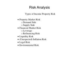
8. General Risk Categories Business Risk – the chance of loss associated with a given managerial decision; typically a by-product of the unpredictable variation in product demand and cost conditions Market Risk – the chance that a portfolio of investments can lose money because of overall swings in financial markets Inflation Risk – the danger that a general increase in the price level will undermine the real economic value of corporate agreements Interest-rate Risk – another type of market risk that can affect the value of corporate investments and obligations Credit Risk – the chance that another party will fail to abide by its contractual obligations

9. General Risk Categories (Con’t.) Liquidity Risk – the difficulty of selling corporate assets or investments that have only a few willing buyers or are otherwise not easily transferable at favorable prices under typical market conditions Derivative Risk – the chance that volatile financial derivatives such as commodity futures and index options could create losses by increasing rather than decreasing price volatility Currency Risk – the chance of loss due to changes in the domestic currency value of foreign profits

10. Probability - Probability: likelihood of particular outcome occurring, denoted by p. The number p is always between zero and one. - Frequency: estimate of probability, p=n/N, where n is number of times a particular outcome occurred during N trials. - Subjective probability: If we do not have frequency, we often resort to informed guesses. Subjective probabilities must follow the same rules of the probability calculus, if we are dealing with rational decision-makers.

11. Probability Distribution • Discrete probability distribution: deals with “events” whose “states of nature” are discrete. The “event” is the state of the economy. The “states of nature” are recession, normal, and boom. • Continuous probability distribution: deals with “events” whose “states of nature” are continuous values. The “event” is profits, and the “states of nature” are various profit levels.

12. Payoff Matrix A table that shows outcomes associated with each possible state of nature. Project A more desirable in a recession. Project B more desirable in a boom. In a normal economy, the projects offer the same profit potential. Decision to Make: A firm must choose only one of the two investment projects (choose Project A or Project B). Each calls for an outlay of $10,000.

13. Expected Value • The payoffs of all events: x1, x2, …, xN • The probability of each event: p1, p2, …, pN • Expected value of x: EV(x) is a weighted-average payoff, where the weights are defined by the probability distribution. • Use the payoff matrix in the previous slide, together with the probability of each state of the economy.

14. Expected profit of Project A and B under different economic states of nature

15. Variance and Standard Deviation • Variance and Standard Deviation: measuring risk The payoffs of all events: x1, x2, …, xN The probability of each event: p1, p2, …, pN • Expected value of x: • Variance: • Standard deviation: square root of variance

16. For project A, what are the variance and standard deviation? EV(A) = $5,000 Variance (σ2) = ($4,000-5,000)2 (.2) + ($5,000-$5,000)2 (.6) + ($6,000-$5,000)2 (.2) (σ2) = ($1,000)2 (.2) + ($0)2 (.6) + ($1,000)2 (.2) (σ2) = $400,000 (units are in terms of squared dollars) σA = $632.46 For project B, what are the variance and standard deviation? EV(B) = $5,400 Variance (σ2) = ($0-5,400)2 (.2) + ($5,000-$5,400)2 (.6) + ($12,000-$5,400)2 (.2) (σ2) = 5,832,000 + 96,000 + 8,712,000 (units are in terms of squared dollars) (σ2) = 14,640,000 (units are in terms of squared dollars) σB = $3,826.23 Project B has a larger standard deviation; therefore it is the riskier project

17. Risk Measurement • Absolute Risk: - Overall dispersion of possible payoffs - Measurement: variance, standard deviation - The smaller variance or standard deviation, the lower the absolute risk. • Relative Risk - Variation in possible returns compared with the expected payoff amount - Measurement: coefficient of Variation (CV), - The lower the CV, the lower the relative risk.

18. Project A EV(A) = $5,000 σA = $632.46 Project B EV(B) = $5,400 σ B = $3,826.23 Coefficient of variation CVA = = 0.1265 CVB = = 0.7086 Coefficient of variation measures the relative risk; the variation in possible returns compared with the expected payoff amount.

19. Risk Attitudes Risk Aversion characterizes decision makers who seek to avoid or minimize risk. Risk Neutrality characterizes decision makers who focus on expected returns and disregard the dispersion of returns. Risk Seeking (Taking) characterizes decision makers who prefer risk.

20. Risk Attitudes Scenario: A decision maker has two choices, a sure thing and a risky option, and both yield the same expected value. Risk-averse behavior: Decision maker takes the sure thing Risk-neutral behavior: Decision maker is indifferent between the two choices Risk-loving (or seeking) behavior: Decision maker takes the risky option

21. Utility Theory and Risk Analysis Typically, consumers and investors display risk-averse behavior, especially when substantial sums of money are involved. Risk aversion is the general assumption behind decision models in managerial economics. Examples to the contrary: State-run lotteries Casinos (gaming) Today, U.S. consumers spend more on legal games of chance than on movie theaters, books, amusement attractions, and recorded music combined! Source: Wall Street Journal, Ann Davis, September 23, 2004.

22. Risk Attitudes (MU) (MU) (MU) Risk averter: diminishing MU Risk neutral: constant MU Risk lover: increasing MU

23. Examples of utility functions • Let w = income (or profit) or more generally wealth, w > 0 Which utility function is consistent with risk-seeking behavior? Which utility function is consistent with risk neutrality? Which utility function is consistent with risk aversion?

24. Under risk aversion behavior, the decision rule is to maximize expected utility. EV[U(risky option)] = U(w1)p1 + U(w2)p2 + U(wn)pn Also, it is important to find the level of income, profits, or wealth that is consistent with the utility level of the expected value of utility associated with the risky option. Call this level of wealth w*. The difference between the expected value of the risky option and w* is the risk premium. Risk premium = EV(risky option) – w*

25. Example: Joshua lives in San Francisco, CA, where the probability of an earthquake is 10%. Suppose that Joshua’s utility function is given by , where w represents total wealth. If Joshua chooses not to buy insurance next year, his wealth is $500,000 if no earthquake occurs, and $300,000 if an earthquake occurs. The reduction in wealth is attributable to the loss of his house due to the earthquake. The risky option is not buying insurance. (a) Is Joshua risk averse, risk loving, or risk neutral? (b) Find the EV of not buying insurance (the risky option). (c) Find EV[U(risky option)]. (d) Find the wealth that results in the utility level associated with the expected value of utility of the risky option. (e) Find the risk premium.

26. Is Joshua risk averse, risk loving, or risk neutral? • MU diminishes with increases in w. • Joshua is risk averse • (b) Find the EV of not buying insurance. • EV(risky option) = ($500,000)(.9) + ($300,000)(.1) = $480,000 • (c) Find EV[U(risky option)]. • EV[U(risky option)] = • EV[U(risky option)] = $636.40 + $54.77 = $691.71 • (d) What level of wealth is consistent with the utility level of the EV[U(risky option)]? • Risk premium. • EV(risky option) – w* = $480,000 - $477,716 • Risk premium = $2,284.

27. Graphical Analysis Utility U= U(500,000) = 707.11 0.9U(500,000) + 0.1U(300,000) = 691.17 U(300,000) = 547.72 Wealth 300,000 477,716 480,000 500,000 risk premium

28. Decision-Making Under Risk • Possible Criteria to consider: - Maximize expected value - Minimize variance or standard deviation - Minimize coefficient of variation - Incorporate risk attitudes: certainty equivalent - Maximin criterion

29. Maximizing Expected Value • EV(A)=$5,000 EV(B)=$5,400 • Thinking: • Which project will you choose based on this criterion? • What is ignored using this criterion?

30. Minimizing Variance/Standard Deviation • = $632.46 = $3,826.23 • Thinking: • Which project will you choose based on this criterion? • What is ignored using this criterion?

31. Coefficient of Variation: Standard Deviation Divided by the Expected Value • Think: • Which project will you choose based on this criterion? • What is ignored?

32. Incorporating Risk Attitudes: Certainty Equivalent Suppose that you face the following choices: (1) Invest $100,000 From a successful project you receive $1,000,000. If the project fails, you receive $0. The probability of success is 0.5. EV(investment) = ($1,000,000)(0.5) + ($0)(.5) = $500,000. (2) You do not make the investment and keep $100,000. If you find yourself indifferent between the two alternatives, $100,000 is your certainty equivalent for the risky expected return of $500,000. A certain or riskless amount of $100,000 provides exactly the same utility as a 50/50 chance to earn $1,000,000 (or $0).

33. In general, any risky investment with a certainty equivalent less than the expected dollar value indicates risk aversion. In our case, $100,000 < $500,000 => risk aversion. Certainly Equivalent Adjustment Factor = = Equivalent Certain Sum Expected Value of the Risky Venture In our case, = $100,000 = .2. $500,000 The “price” of one dollar in this risky venture is equal to 20¢ in certain dollar terms.

34. = Equivalent Certain Sum Expected Value of the Risky Venture If Then Implies Equivalent certain sum < Expected Value of the < 1 Risk aversion Risky Venture Equivalent certain sum = Expected Value of the = 1 Risk indifference Risky Venture (or neutrality) Equivalent certain sum > Expected Value of the > 1 Risk preference Risky Venture (or taking)

35. Game Theory - Game Theory dates back to the 1940s by John von Neuman (Mathematician) and Oskar Morgenstern (Economist) - Game Theory is a useful decision framework employed to make choices in hostile environments and under extreme uncertainty. - Use of maximin decision rule - Use of minimax regret decision rule (opportunity loss).

36. Maximin Decision Rule The decision maker should select the alternative that provides the best of the worst possible outcomes. Maximize the minimum possible outcome. The maximin criterion focuses only on the most pessimistic outcome for each decision alternative. The maximin criterion implicitly assumes a very strong aversion to risk and is quite appropriate for decisions involving the possibility of catastrophic outcomes.

37. Minimax Regret Decision Rule This decision rule focuses on the opportunity loss associated with a decision rather than on its worst possible outcome. The decision maker should minimize the maximum possible regret (opportunity loss) associated with a wrong decision after the fact. Minimize the difference between possible outcomes and the best outcome for each state of nature. Opportunity loss => the difference between a given payoff and the highest possible payoff for the resulting state of nature. So, find the maximum payoff for a given state of nature and then subtract from this amount the payoffs that would result from various decision alternatives.

38. Maximin and Minimax Regret Decision Rules • Thinking: • Which project will you choose? - Based on Maximin Decision Rule? - Based on Minimax Regret Decision Rule? • What is ignored in the respective decisions?

39. Maximin Decision Rule Example Minimum possible outcome for project A is $4,000. Minimum possible outcome for project B is $0. Therefore by the maximin decision rule, choose project A.

40. Minimax Regret Decision Rule Calculate the opportunity loss or regret matrix Therefore, by the minimax regret decision rule, choose project B.

41. What’s Next? • Preparation for Exam I • Exam I Covers: - Algebra review - Demand analysis - Risk analysis