Download
1 / 56
560 likes | 651 Vues
Explore the impact of subdiffusive nature on reaction dynamics in (sub)diffusion limited reactions, with a focus on subordination. Learn through examples and simulations.

E N D
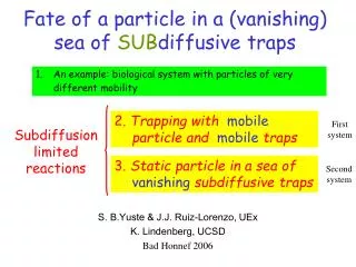
Fate of a particle in a (vanishing) sea of SUBdiffusive traps • An example: biological system with particles of very different mobility 2. Trapping with mobile particle and mobile traps First system Subdiffusion limited reactions S. B.Yuste & J.J. Ruiz-Lorenzo, UEx K. Lindenberg, UCSD Bad Honnef 2006 3. Static particle in a sea of vanishing subdiffusive traps Second system
“Visualization and Tracking of Single Protein Molecules in theCell Nucleus”, Kues, Peters, and Kubitscheck, Biophysical Journal, 80 (2001) 2954 Very different mobilities!
“Visualization and Tracking of Single Protein Molecules in theCell Nucleus”, Kues, Peters, and Kubitscheck, Biophysical Journal, 80 (2001) 2954 “Using the comparatively “inert” recombinant protein, P4K, we observed only diffusional motion. However, within this category a range of modes was detected. Thus one population of molecules appeared to be immobile ... while at least three different mobile fractions were detected. Two of the mobile fractions, fmob,1 and fmob, 2, were analyzed quantitatively in terms of time dependent diffusion coefficients.... However, the diffusion coefficient of fraction fmob,2 was also decreasing with time. The third mobile fraction, fmob,3, of ;5% moves very fast with jump...” subdiffusion!
The general problem: What are the consequences of the subdiffusive nature of the reactants on the reaction dynamics of (sub)diffusion limited reactions? ● A bumpy road: generalization of the usual reaction-diffusion equations κ Example: A → Bin one dimension(Sokolov, Schmidt, Sagués, PRE, 73 (2006)) Subdiffusive reactants Diffusive reactants Generalization
The general problem: What are the consequences of the subdiffusive nature of the reactants on the reaction dynamics of (sub)diffusion limited reactions? ●A bumpy road: generalization of the usual reaction-diffusion equations ● An easy (but qualitative) answer: Subordination : What is relevant in reaction dynamics is h x2iso that... h x2i» t h x2i» t t! t diffusion limited reactions subdiffusion limited reactions • ...but not always true: • Long-time reaction rate in the subdiffusive trapping problem» 1/t • Long-time reaction rate in the diffusive trapping problem» exp(- t1/3) ? Donsker-Varadhan
Particle in a 1D sea of subdiffusive traps : 1D subdiffusion limited reactions whereA ☞Objective: reaction dynamics ⇔ survival probability P(t) Particle in a 1D sea of subdiffusive traps ☑ 1. Target problem: A(static)+T→T Yuste&Acedo Physica A 336, 334 (2004) Yuste&Acedo Physica A 336, 334 (2004) 2. Trapping problem: A+T(static) →T(static) ☑ ☞ 3. A+T→T (A & T mobile) Yuste&Lindenberg, PRE 72, 061103 (2005)
Particle in a sea of traps 1D Long-time reaction dynamics Recapitulation A mobile T static A mobile T mobile Donsker-Varadhan Bramson-Lebowitz Diffusion Bray-Blythe Blumen-Klafter-Zumofen ??????? Subdiffusion ☞Our first problem
A rigorous approach ...to the problem ofSUBdiffusive particle in a sea of SUBdiffusive traps To find lower and upper bounds for P(t): PL(t) ≤ P(t) ≤ PU(t) where, for t→∞, PL(t) → P(t) ←PU(t) A successfulapproach for normal diffusion (Bray & Blythe, PRL 2001)
Yuste&Lindenberg, PRE 72, 061103 (2005) For a subdiffusive particle ( 0< γ’ < 1 )and subdiffusive or diffusive traps ( 0< γ≤ 1 ) t → ∞ 0 For a diffusive particle (γ’ = 1) and subdiffusive trapswith2/3 < γ≤ 1 t → ∞ 0 Target problem P(t) ! t!tγ subordination☑ P(t)»exp(-4 /1/2 D1/2 t1/2)
Survival probabilityof a (SUB)diffusive particle in a sea of (SUB)diffusive traps Normal diffusion Bramson-Lebowitz, Bray-Blythe 1. Exact result for the green region Donsker-Varadhan Diffusive particle (γ’=1) in a sea of strongly (γ<2/3)SUBdiffusive traps
Survival probabilityof a (SUB)diffusive particle in a sea of (SUB)diffusive traps Normal diffusion Bramson-Lebowitz, Bray-Blythe 1. Exact result for the green region λbounded but unknown Donsker-Varadhan Diffusive particle (γ’=1) in a sea of strongly (γ<2/3)SUBdiffusive traps
For a diffusive particle (γ’ = 1)and subdiffusive traps withγ < 2/3 PL(t) ≤ P(t) ≤ PU(t) ∞ t → ∞ subordination?
Survival probabilityof a (SUB)diffusive particle in a sea of (SUB)diffusive traps Normal diffusion Bramson-Lebowitz, Bray-Blythe Exact result for the green region λbounded but unknown ? or No exact prediction for the orange line Donsker-Varadhan Diffusive particle (γ’=1) in a sea of strongly (γ<2/3)SUBdiffusive traps
Simulation results for the exponent θ: θ=1/2 Bramson-Lebowitz □ (0.5,1) 1 □ (0.8,0.8) □ (1.0,0.8) □ (0.4,0.8) θ=1/3 2/3 θ= γ/2 γ 1/3 ? γ/2 (subord.) ? θ= □ (0.9,0.5) □ (0.4,0.4) □ (0.5,0.4) □ (1.0,0.4) □ (0.6,0.4) □ (0.7,0.4) Diffusive particle (γ’=1) in a sea of strongly (γ<2/3)SUBdiffusive traps 0 1 θ=1/3 Donsker-Varadhan 0 γ’
Subdiffusive particle ( 0< γ’ < 1 )and subdiffusive traps ( 0< γ<1 ) OK! Case γ’=0.4 , γ=0.4 : Exponent θ ⇔ P(t)=1.4E-06 ρ=0.01 γ=0.4 (trap) γ’=0.4 (part.) L=10^4 P(t)=6.2E-04 ☑ Exponent θ θ=0.2 (Simu.) θ=γ/2 (Theo.) P(t)=0.034
Subdiffusive particle ( 0< γ’ < 1 )and diffusive traps ( γ= 1 ) OK! Case γ’=0.5 , γ=1 : Exponent θ ⇔ P(t)=5.1E-06 ρ=0.01 γ=1 (trap) γ’=0.5 (part.) L=10^4 θ=0.5 (Simu.) θ=γ/2 (Theo.) P(t)=0.37 ☑ Exponent θ
Subdiffusive particle ( 0< γ’ < 1 )and subdiffusive traps ( 0< γ≤ 1 ) OK! Case γ’=0.4 , γ=0.8 : Exponent θ ⇔ P(t)=5.1E-06 rho_0=0.1 θ_simu=0.38 rho_0=0.01 θ_simu=0.39 θ_teo=γ/2=0.4 P(t)=0.37
Subdiffusive particle ( 0< γ’ < 1 )and subdiffusive traps ( 0< γ≤ 1 ) OK! Case γ=0.8, γ’=0.8 : Exponent θ ⇔ rho_0=0.1 θ_simu=0.37 rho_0=0.01 θ_simu=0.38 θ_teo=γ/2=0.4
Simulation results for the exponent θ: 1 θ=1/2 Bramson-Lebowitz ☺ (0.5,1) ☺ (0.8,0.8) □ (1.0,0.8) ☺ (0.4,0.8) θ=1/3 2/3 θ= γ/2 γ □ (0.9,0.5) 1/3 ? γ/2 (subord.) ? θ= ☺ (0.4,0.4) □ (0.5,0.4) □ (1.0,0.4) □ (0.6,0.4) □ (0.7,0.4) □ (0.8,0.4) Diffusive particle (γ’=1) in a sea of strongly (γ<2/3)SUBdiffusive traps 0 θ=1/3 Donsker-Varadhan 1 0 γ’
Subdiffusive particle ( 0< γ’ < 1 )and subdiffusive traps ( 0< γ≤ 1 ) ? Case γ’=0.5 , γ=0.4 : Exponent θ ⇔ rho_0=0.1 θ_simu=0.18 rho_0=0.01 θ_simu=0.15 θ_teo=γ/2=0.2
Diffusive particle (γ’= 1 )and subdiffusive traps with 2/3 < γ ≤ 1 ? Case γ’=1, γ=0.8 : Exponent θ ⇔ P(t)=5.1E-06 rho_0=0.01 θ_simu=0.45 P(t)=0.37 θ_teo=γ/2=0.4
Simulation results for the exponent θ: 1 θ=1/2 Bramson-Lebowitz ☺ (0.5,1) ☺ (0.8,0.8) (1.0,0.8) ☺ (0.4,0.8) θ=1/3 2/3 θ= γ/2 γ 1/3 ? γ/2 (subord.) ? θ= □ (0.9,0.5) ☺ (0.4,0.4) □ (1.0,0.4) □ (0.6,0.4) □ (0.7,0.4) (0.5,0.4) Diffusive particle (γ’=1) in a sea of strongly (γ<2/3)SUBdiffusive traps 0 1 θ=1/3 Donsker-Varadhan 0 γ’
Subdiffusive particle ( 0< γ’ < 1 )and subdiffusive traps ( 0< γ≤ 1 ) ? Case γ’=0.6 , γ=0.4, : Exponent θ ⇔ rho_0=0.1 θ_simu=0.18 rho_0=0.01 θ_simu=0.13 θ_teo=γ/2=0.2
Subdiffusive particle ( 0< γ’ < 1 )and subdiffusive traps ( 0< γ≤ 1 ) ? Case γ’=0.7 , γ=0.4 : Exponent θ ⇔ rho_0=0.5 θ_simu=0.18 rho_0=0.1 θ_simu=0.12 θ_teo=γ/2=0.2
Subdiffusive particle ( 0< γ’ < 1 )and subdiffusive traps ( 0< γ≤ 1 ) ? Case γ’=0.9 , γ=0.5 : Exponent θ ⇔ rho_0=0.5 θ_simu=0.27 rho_0=0.01 θ_simu=0.12 rho_0=0.1 θ_simu=0.19 θ_teo=γ/2=0.25
Exponent θ: 1 θ=1/2 Bramson-Lebowitz ☺ (0.5,1) ☺ (0.8,0.8) (1.0,0.8) ☺ (0.4,0.8) θ=1/3 2/3 θ= γ/2 γ 1/3 ? γ/2 (subord.) ? θ= ☹ (0.9,0.5) ☺ (0.4,0.4) □ (1.0,0.4) ☹ (0.6,0.4) (0.5,0.4) ☹ (0.7,0.4) Diffusive particle (γ’=1) in a sea of strongly (γ<2/3)SUBdiffusive traps 0 1 θ=1/3 Donsker-Varadhan 0 γ’
Diffusive particle ( γ’ = 1 )and subdiffusive traps ( γ <2/3 ) ? Case γ=0.4, γ’=1 : Exponent θ ⇔ rho_0=0.5 θ_simu=0.47 rho_0=0.1 θ_simu=0.43 θ_teo={1/3,γ/2=0.2}
Simulation results for the exponent θ: 1 θ=1/2 Bramson-Lebowitz ☺ (0.5,1) ☺ (0.8,0.8) (1.0,0.8) ☺ (0.4,0.8) θ=1/3 2/3 θ= γ/2 γ γ/2 (subord.) ? 1/3 ? θ= ☹ (0.9,0.5) ☺ (0.4,0.4) (1.0,0.4) ☹ (0.6,0.4) (0.5,0.4) ☹ (0.7,0.4) Okay, you win, I can't drive a ship... Diffusive particle (γ’=1) in a sea of strongly (γ<2/3)SUBdiffusive traps Simulation´s Bermuda triangle 0 1 θ=1/3 Donsker-Varadhan 0 γ’
Making sense (?) of simulations results for 1 ☺ Theo. ? γ ? ☹ 0 1 γ’ 0 • Simulations for ’ > are inconclusive: • exponent θnot well-defined • Simulations for ’ ≤ are conclusive: • exponent θ =γ/2 robust Why ? for t→∞ Static particle Mobile traps Fast particle ’ > Slow traps Target problem Hard for simulations!!
☞Static particle in a 1D sea ofvanishing(sub)diffusive traps T → Ø A + T → T static + t1 : r(t1) t2 : r(t2)< r(t1) What is the survival probability P(t) of the particle?
An exact integral equation for P(t)=exp[-μ0(t)] Bray, Majumdar, Blythe , PRE 67, 060102R (2003) t! 0 t=t-t’ x x t t’ t t’ Probability that a trap has met the particle in the time interval (t',t'+dt') for the first time Probability density to find a trap at x=0 at time t the probability density for this particular trap to be again at x=0 at time t. the probability of a trap surviving till time t, given that it survives till time t’ For subdiffusive traps:
The final integral equation Tautochrone is the famous (generalized) Abel’s integral equation. The solution is: Inverse problem prescribed
Exponentially vanishing sea of traps = trap’s mean timelife typical length explored by a trap before vanishing 0-1= typical distance between traps at t=0 … eternal life! !1 Classic target problem Normal diffusive traps, =1 Yuste&Acedo Physica A 336, 334 (2004) ☑ Subordination: t! t
Survival probability for normal diffusive traps with 0 =0.001, τ=105 - ln P(t) time
Survival probability for subdiffusive traps with γ= ½, ρ0 =0.01, τ=108 - ln P(t) time
Power-law vanishing sea of traps For t!1 : /2< /2= /2> typical length explored by a trap»t/2 mean distance between traps»-1»t
Survival probability for subdiffusive traps with γ= 0.75, =0.4, =106, ρ0 =0.01 γ/2< - ln P(t) time
Survival probability for subdiffusive traps with γ= 0.8, =0.4, =106, ρ0 =0.01 γ/2= - ln P(t) time
Survival probability for subdiffusive traps with γ= 0.8, =0.2, =106, ρ0 =0.01 γ/2> - ln P(t) time
Remarks and conclusions: • Systems with reactive particles of very disparate diffusivities do exist and are worth studying. • First steps into the study of subdiffusion-limited reactions with reactive species with different anomalous diffusion exponents. • Long-time reaction dynamics regime for subdiffusive particles in a sea of subdiffusive traps inaccessible by simulation methods when γ’>γ. • “Long-time” reaction dynamics regime for subdiffusive particles in a sea of subdiffusive traps reached very soon when γ’<γ. • .Exact solution for a class of a subdiffusion-limited reactions: the target problem with arbitrarytime-dependent density of traps. ... andsome open problems • What is the survival probability of a diffusive particle in a sea of strongly (γ < 2/3 ) SUBdiffusive traps? • Reaction dynamics for a subdiffusive particle in a sea of vanishing subdiffusive traps. • To improve simulations (better methods?) • To extend the results to higher dimensions (d=2, d=3). • Intermediate-time reaction dynamics (specially for γ’>γ) .
The general problem: What are the consequences of the subdiffusive nature of the reactants on the reaction dynamics of (sub)diffusion limited reactions? ● A bumpy road: generalization of the reaction-diffusion equation κ Example: A → Bin one dimension(Sokolov, Schmidt, Sagués, PRE, 73 (2006)) Subdiffusive reactants Diffusive reactants Generalization
● An easy (but qualitative) answer: Subordination : What is relevant is h x2iso that... h x2i» t h x2i» t t! t diffusion limited reactions subdiffusion limited reactions • ...but not always true: • Long-time reaction rate in the subdiffusive trapping problem» 1/t • Long-time reaction rate in the diffusive trapping problem» exp(- t1/3) Donsker-Varadhan ?
An idea... 1. We have seen that P(t)»exp(-4 /1/2 D1/2 t1/2) , t !1 for the full diffusive caseγ’ =γ=1 2. Qualtitatively, in many cases, one can getthe subdiffusive behavior from the diffusive one by means of the changet ! tγ(“subordination”) So that for SUBdiffusive particle in a sea of SUBdiffusive traps … Hypothesis: P(t)»exp(-const. K1/2tγ/2) , t !1
Blue line: Black line: erfc(t/2)
An open problem:Diffusive particle (γ’=1) in a sea ofstrongly (γ < 2/3)SUBdiffusive traps θ 1/2 ? θ=1/3 Donsker-Varadhan exponent for the trapping problem: diffusive particle in a sea of static (γ→0) traps ● 1/3 ? Subordination 0 γ 0 1 1/3 2/3
Last minute message A closely related problem studied in : Kinetics of Trapping Reactions with a Time Dependent Density of Traps Alejandro D. Sánchez, Ernesto M. Nicola, and Horacio S. Wio Phys. Rev. Lett.78, 2244–2247 (1997) ... but different: • Involve three normal diffusive species • Different approach • Approximate expressions • No subdiffusion
Subdiffusive particle ( 0< γ’ < 1 )and subdiffusive traps ( 0< γ< 1 ) Case γ’=0.4 , γ=0.4: Prefactor λ γ=0.4 (trap) γ’=0.4 (part.) L=10^4 ρ=0.1 (red) ρ=0.01 (green) ☑ Prefactor λ
Subdiffusive particle ( 0< γ’ < 1 )and diffusive traps ( 0< γ≤ 1 ) Case γ’=0.5 , γ=1 : Prefactor λ ☑ Prefactor λ ρ=0.01 γ=1 (trap) γ’=0.5 (part.) L=10^4


![❤[PDF]⚡ Vanishing Twins: A Marriage](https://cdn7.slideserve.com/13194511/slide1-dt.jpg)