Chapter 8 Large-Sample Estimation
Chapter 8 Large-Sample Estimation. General Objectives:

Chapter 8 Large-Sample Estimation
E N D
Presentation Transcript
Chapter 8 Large-Sample Estimation General Objectives: This chapter presents a method for estimating population parameters and illustrates the concept with practical examples. The Central Limit Theorem and the sampling distributions presented in Chapter 7 play a key role in evaluating the reliability of the estimates. ©1998 Brooks/Cole Publishing/ITP
Specific Topics 1. Types of estimators 2. Picking the best point estimator 3. Point estimation for a population mean or proportion 4. Interval estimation 5. Large-sample confidence intervals for a population mean or proportion 6. Estimating the difference between two population means 7. Estimating the difference between two binomial proportions 8. One-sided confidence bounds 9. Choosing the sample size ©1998 Brooks/Cole Publishing/ITP
8.1 Where We’ve Been Descriptive Statistics Probability and Probability Distributions Binomial and Normal Distributions Link Between Probability and Statistical Inference The Central Limit Theorem Populations Statistics Inferential Statistics ©1998 Brooks/Cole Publishing/ITP
8.2 Where We’re Going— Statistical Inference • Applications of inference: - The government needs to predict short- and long-term interest rates. - A broker wants to forecast the behavior of the stock market - A metallurgist wants to decide whether or new type of steel is more resistant to high temperatures than the old type was. - A consumer wants to estimate the selling price of her house before putting it on the market. • Statistical inference is concerned with making decisions or predictions about parameters. ©1998 Brooks/Cole Publishing/ITP
Methods for making inferences about population parameters fall into one of two categories: - Estimation: Estimating or predicting the value of the parameter - Hypothesis testing: Making a decision about the value of a parameter based on some preconceived idea about what its value might be • Examples 8.1 and 8.2 give illustrations of estimation and hypothesis testing problems respectively. • Statistical procedures are important because they provide two types of information: - Methods for making the inference - A numerical measure of the goodness or reliability of the inference. ©1998 Brooks/Cole Publishing/ITP
Example 8.1 The circuits in computers and other electronics equipment consist of one or more printed circuit boards (PCB), and computers are often repaired by simply replacing one or more defective PCBs. In an attempt to find the proper setting of a plating process applied to one side of a PCB, a production supervisor might estimate the average thickness of copper plating on PCBs using samples from several days of operation. Since he has no knowledge of the average thickness m before observing the production process, his is an estimation problem. ©1998 Brooks/Cole Publishing/ITP
8.3 Types of Estimators Definition: An estimator is a rule, usually expressed as a formula, that tells us how to calculate an estimate based on information in the sample. • Estimators are used in two different ways: - Point estimation: Based on sample data, a single number is calculated to estimate the population parameter. The rule or formula that describes this calculation is called the point estimator, and the resulting number is called a point estimate. - Interval estimation: Based on sample data, two numbers are calculated to form an interval within which the parameter is expected to lie. ©1998 Brooks/Cole Publishing/ITP
The rule or formula that describes this calculation is called theinterval estimator, and the resulting pair of numbers is called aninterval estimate or confidence interval. • Example 8.3 discusses a possible estimator based on sample data. Example 8.3 A veterinarian wants to estimate the average weight gain per month of 4-month-old golden retriever pups that have been placed on a lamb and rice diet. The population consists of the weight gains per month of all 4-month-old golden retriever pups that are given this particular diet. Hence, it is a hypothetical population where m is the average monthly weight gain for all 4-month-old golden retriever pups on this diet. This is the unknown parameter that the veterinarian wants to estimate. One possible estimator based on sample data is the sample mean, ©1998 Brooks/Cole Publishing/ITP
It could be used in the form of a single number or point estimate—for instance, 3.8 pounds—or you could use an interval estimate and estimate that the weight gain will fall into an interval such as 2.7 to 4.9 pounds. ©1998 Brooks/Cole Publishing/ITP
8.4 Point Estimation • Point estimation is used in estimating population means and proportions. • To choose the best statistic or estimator, observe their behavior in repeated sampling, described by their sampling distributions. • Two characteristics are valuable in a point estimator: 1. The sampling distribution of the point estimator should be centered over the true value of the parameter to be estimated. 2. The spread (as measured by the variance) of the sampling distribution should be as small as possible. • Figure 8.1 illustrates differences in centering and spread for sampling distributions. ©1998 Brooks/Cole Publishing/ITP
Figure 8.1 ©1998 Brooks/Cole Publishing/ITP
Definition: An estimator is said to be unbiased if the mean of its distribution is equal to the true value of the parameter. Otherwise, the estimator is said to be biased. • Figure 8.2 shows distributions for biased and unbiased estimators. Figure 8.3 compares estimator variability. Definition: The distance between an estimate and the estimated parameter is called the error of estimation. Figure 8.2 ©1998 Brooks/Cole Publishing/ITP
Point Estimation of a Population Parameter: - Point estimator: A statistic calculated using sample measurements - Margin of error: 1.96 ´ Standard error of the estimator. • Figure 8.4 shows the sampling distribution of an unbiased estimator. Figure 8.4 ©1998 Brooks/Cole Publishing/ITP
Estimating a population mean or proportion: • To estimate the population mean m for a quantitative population, the point estimator is unbiased with standard error given as - The margin of error is calculated as - If s is unknown and n is 30 or larger, the sample SD s can be used to approximate s. • To estimate the population proportion p for a binomial population, the point estimator is unbiased with standard error given as . - The margin or error is calculated as and estimated as ©1998 Brooks/Cole Publishing/ITP
Assumptions: np > 5and nq > 5. Since p and q are unknown, use • Table 8.1 displays some calculated values of Examples 8.4 and 8.5 estimate the population mean and the population proportion, respectively. • In calculating the standard error for these two point estimates, you need to estimate s with s, p with and q with Table 8.1 p pq p pq .1 .09 .30 .6 .24 .49 .2 .16 .40 .7 .21 .46 .3 .21 .46 .8 .16 .40 .4 .24 .49 .9 .09 .30 .5 .25 .50 ©1998 Brooks/Cole Publishing/ITP
Example 8.4 An investigator is interested in the possibility of merging the capabilities of television and the Internet. A random sample of n= 50 Internet users who were polled about the time they spend watching television produced an average of 11.5 hours per week with a standard deviation of 3.5 hours. Use this informa-tion to estimate the population mean time Internet users spend watching television. Solution The random variable measured is the time spent watching television per week. This is a quantitative random variable best described by its mean m. The point estimate of m, the average time Internet users spend watching television, is hours. The margin of error is ©1998 Brooks/Cole Publishing/ITP
Although s is unknown, the sample size is large, and you can approximate the value of s by using s. Therefore, the margin of error is approximately You can feel fairly confident that the sample estimate of 11.5 hours of television watching for Internet users is within ±1 hour of the population mean. ©1998 Brooks/Cole Publishing/ITP
Figure 8.5 Plot of treatment means and their standard errors ©1998 Brooks/Cole Publishing/ITP
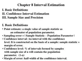
8.5 Interval Estimation • An interval estimator is a rule for calculating two numbers—say, a and b—that create an interval that you are fairly certain contains the parameters of interest, e.g., a confidence interval. • The concept of “fairly certain” can be quantified using a statistical concept called the confidence coefficient and designated by (1- a). Definition: The probability that a confidence interval will contain the estimated parameter is called the confidence coefficient. Constructing a Confidence Interval: - For the standard normal random variable z, 95% of all values lie between -1.96 and 1.96. ©1998 Brooks/Cole Publishing/ITP
Figure 8.6 shows the 95% confidence limits for a population parameter. • Figure 8.7 displays the locations of za/2. Table 8.2 displays values of z commonly used. Figure 8.6 95% confidence limits for a population parameter ©1998 Brooks/Cole Publishing/ITP
Figure 8.7 Location of za/2 ©1998 Brooks/Cole Publishing/ITP
- For an unbiased point estimator with a normal sampling distribution, 95% of all point estimates lie with 1.96 standard errors of the parameter of interest. - Consider constructing the interval as: point estimate ± 1.96SE. As long as the point estimate is within 1.96SE of the parameter of interest, the interval centered at this estimate will contain the parameter of interest. This will happen 95% of the time. • You may want to change the confidence coefficient from (1- a) = .95 to another confidence level (1- a). To do this, you will need to adjust the z-value. A (1- a)100% Large-Sample Confidence Interval: where za/2 is the z-value with an area of a/2 in the right tail of a standard normal distribution. This formula generates two values; the lower confidence limit (LCL) and the upper confidence limit (UCL). ©1998 Brooks/Cole Publishing/ITP
A (1- a)100% Large-Sample Confidence Interval for a Population Mean m: where za/2 is the value corresponding to an area a/2 in the upper tail of a standard normal z distribution, and n = Sample size s= Standard deviation of the sampled population. If s is unknown, it can be approximated by the sample standard deviation s when the sample size is large (n > 30) and the approximate confidence interval is • Example 8.6 constructs a 95% confidence interval for the mean daily intake of dairy products for men. ©1998 Brooks/Cole Publishing/ITP
Example 8.6 A scientist interested in monitoring chemical contaminates in food, and thereby the accumulation of contaminates in human diets, selected a random sample of n= 50 male adults. It was found that the average daily intake of dairy products was grams per day with a standard deviation of s= 35 grams per day. Use this sample information to construct a 95% confidence interval for the mean daily intake of dairy products for men. Solution Since the sample size of n= 50 is large, the distribution of the sample mean is approximately normally distributed with mean m and standard error Since the population standard deviation is unknown, you can use the sample standard deviation s as its best estimate. ©1998 Brooks/Cole Publishing/ITP
The approximate 95% confidence interval is Hence, the 95% confidence interval for m is from 746.30 to 765.70 grams per day. • Interpreting the Confidence Interval: 95% of the confidence intervals constructed using different sample information would contain within their upper and lower bounds. ©1998 Brooks/Cole Publishing/ITP
Figure 8.8 shows 20 confidence intervals for the mean for Example 8.6. • Example 8.7 constructs a 99% confidence interval for the mean daily intake of dairy products for adult men in Example 8.6. • Figure 8.10 shows the sampling distributions for based on random samples for a normal distribution with n = 5, 20, and 80. ©1998 Brooks/Cole Publishing/ITP
Figure 8.8 Twenty confidence intervals for the mean for Example 8.6 ©1998 Brooks/Cole Publishing/ITP
Example 8.7 Construct a 99% confidence interval for the mean daily intake of dairy products for adult men in Example 8.6. Solution To change the confidence level to .99, you must find the appropriate value of the standard normal z that puts area(1 - a) = .99 in the center of the curve. This value, with tail area a/2 = .005 to its right, is found from Table 8.2 to be z= 2.58. The 99% confidence interval is then ©1998 Brooks/Cole Publishing/ITP
Large-Sample Confidence Interval for a Population Proportion p - When the sample size is large, the sample proportion, - The sampling distribution is approximately normal, with mean p and standard error A (1- a)100% Large-Sample Confidence Interval for a Population Proportion p where za/2 is the z-value corresponding to an area a/2 in the right tail of a standard normal z distribution. Estimate p and q with Sample size is considered large when np > 5and nq > 5. ©1998 Brooks/Cole Publishing/ITP
8.6 Estimating the Difference Between Two Population Means • Table 8.3 shows how the estimates of the population parameters are calculated from the sample data. Properties of the Sampling Distribution of ,the Difference Between Two Sample Means: • When independent random sample of n1 and n2 have been selected from populations with means m1 and m2 and variances, respectively, the sampling distribution of the differences has the following properties: 1. The mean and the standard error of are and ©1998 Brooks/Cole Publishing/ITP
2. If the sampled populations are normally distributed, then the sampling distribution of is exactly normally distributed, regardless of the sample size. 3. If the sampled populations are not normally distributed, then the sampling distribution of is approximately normally distributed when n1 and n2 are large, due to the CLT. • Since m1-m2 is the mean of the sampling distribution, is an unbiased estimator of (m1-m2 ) with an approximately normal distribution. • The statistic has an approximately standard normal z distribution. ©1998 Brooks/Cole Publishing/ITP
Point Estimation of (m1-m2 ): Point estimator: Margin of error: • If are unknown, but both n1 and n2 are 30 or more, you can use the sample variances to estimate A (1-a)100% Confidence Interval for (m1-m2 ) : ©1998 Brooks/Cole Publishing/ITP
If are unknown, they can be approximated by the sample variances and the approximate confidence interval is • Example 8.9 illustrates the calculation of confidence intervals. ©1998 Brooks/Cole Publishing/ITP
Example 8.9 The wearing qualities of two types of automobile tires were compared by road-testing samples of n1= n2 = 100 tires for each type. The number of miles until wearout was defined as a specific amount of tire wear. The test results are given in Table 8.4. Estimate (m1-m2), the difference in mean miles to wearout, using a 99% confidence interval. Is there a difference in the average wearing quality for the two types of tires? Solution The point estimate of (m1-m2) is and the standard error of is ©1998 Brooks/Cole Publishing/ITP
where are used to estimate respectively. The 99% confidence interval is calculated as or 824.2 < (m1- m2) < 1775.8. The difference in the average miles to wearout for the two types of tires is estimated to be between LCL = 824.2 and UCL = 1775.8 miles of wear. ©1998 Brooks/Cole Publishing/ITP
Based on this confidence interval, can you conclude that there is a difference in the average miles to wearout for the two types of tires? If there were no difference in the two population means, then m1 and m2 would be equal and (m1 -m2 ) = 0.If you look at the confidence interval you constructed, you will see that 0 is not one of the possible values for (m1 -m2 ). Therefore, it is not likely that the means are the same; you can conclude that there is a difference in the average miles to wearout for the two types of tires. The confidence interval has allowed you to make a decision about the equality of the two population means. ©1998 Brooks/Cole Publishing/ITP
The sampling distribution of has a standard normal distribution for all sample sizes when both sampled populations are normal and an approximate standard normal distribution when the sampled populations are not normal but the sample sizes are large (greater than or equal to 30). • When are not known and are estimated by the sample estimated by the sample estimates the resulting statistic will also have an approximate standard normal distribution when the sample sizes are large. ©1998 Brooks/Cole Publishing/ITP
8.7 Estimating the Difference Between Two Binomial Proportions Properties of the Sampling Distribution of the Difference Between Two Sample Proportions: • Assume that independent random samples of n1 and n2 observations have been selected from binomial populations with parameters p1 and p2, respectively. The sampling distribution of the difference between sample proportions has these properties: 1. The mean and the standard error of are ©1998 Brooks/Cole Publishing/ITP
2. The sampling distribution of can be approximated by a normal distribution when n1 and n2 are large, due to the CLT. • Although the range of a single proportion is from 0 to 1, the difference between two proportions ranges from -1 to +1. • To use a normal distribution to approximate the distribution of , both p1 and p2 should be approximately normal; that is Point estimation of Point estimator: Margin of error : ©1998 Brooks/Cole Publishing/ITP
Note: The estimates must be substituted for p1, p2, q1, and q2 to estimate the margin of error. A (1-a) 100% Large-Sample Confidence Interval for (p1-p2): • Assumption: n1 and n2 must be sufficiently large so that the sampling distribution of can be approximated by a normal distribution—namely, if n1p1, p1q1, n2 p2, and n2q2 are all greater than 5. • Example 8.11 displays the calculation of a confidence interval and the margin of error. ©1998 Brooks/Cole Publishing/ITP
8.8 One-Sided Confidence Bounds • The confidence intervals discussed in Section s 8.5–8.7are sometimes called two-sided confidence intervals because they produce both a UCL and an LCL for the parameter of interest. • Sometimes an experimenter needs only an upper or lower limit. • You can construct a one-sided confidence bound for the parameter of interest, such as m, p, m1- m2., or p1- mp2 . A (1 -a)100% Lower Confidence Bound (LCB): (Point estimator) - za ´ (Standard error of the estimator) A (1 -a)100% Upper Confidence Bound (UCB): (Point estimator) + za ´ (Standard error of the estimator) ©1998 Brooks/Cole Publishing/ITP
The z-value used for a (1 -a)100% one-sided confidence bound, za , locates an area in a single tail of the normal distribution. • Figure 8.11 illustrates a z-value for a one-sided confidence bound. • Example 8.12 finds the 95% upper confidence bound for the mean interest rate that a corporation will have to pay for notes. ©1998 Brooks/Cole Publishing/ITP
8.9 Choosing the Sample Size • The total amount of relevant information in a sample is controlled by two factors: - The sampling plan or experimental design: the procedure for collecting the information - The sample size n: the amount of information you collect • In a statistical estimation problem, the accuracy of the estimation is measured by the margin of error or the width of the confidence interval. • Approximately 95% of the time in repeated sampling, the distance between the sample mean and the population mean m will be less than 1.96SE. ©1998 Brooks/Cole Publishing/ITP
If, for example, you want this quantity to be less than 4, then • Solving for n, you obtain • If you know s, the population standard deviation, you can substitute its value into the formula and solve for n. • If s is unknown—which is often the case—you can use the best approximation available: - An estimate s obtained from a previous sample - A range estimate based on knowledge of the largest and smallest possible measurements: s» Range¤4 • The bound B on the error of your estimate is ©1998 Brooks/Cole Publishing/ITP
Choosing the Sample Size: Determine the parameter to be estimated and the standard error of its point estimator. Then proceed as follows: 1. Choose B, the bound on the error of your estimate, and a confidence coefficient (1-a). 2. For a one-sample problem, solve this equation for the sample size n: za ´ (Standard error of the estimator) =B where za/2 is the value of z having area a/2 to its right. 3. For a two-sample problem, set n1=n2=nand solve the equation in step 2. • Note: For most estimators (all presented in this text), the standard error is a function of the sample size n. • Example 8.13 determines the sample size required for a given bound on error B and probability of error. • Example 8.14 determines the number of workers that must be in each training group for a given B and p. ©1998 Brooks/Cole Publishing/ITP
Example 8.13 Producers of polyvinyl plastic pipe want to have a supply of pipes sufficient to meet marketing needs. They wish to survey wholesalers who buy polyvinyl pipe in order to estimate the proportion who plan to increase their purchases next year. What sample size is required if they want their estimate to be within .04 of the actual proportion with probability equal to .90? Solution For this particular example, the bound B on the error of the estimate is .04. Since the confidence coefficient is (1-a) = .90, a must equal .10 and a/2 is .05. The z-value corresponding to an area equal to .05 in the upper tail of the z distribution is z.05= 1.645. You then require ©1998 Brooks/Cole Publishing/ITP
In order to solve this equation for n, you must substitute an approximate value of p into the equation. You could use the estimate based on the sample of n= 100; or if you want to be certain that the sample is large enough, you could use p= .5 (substituting p= .5 will yield the largest possible solution for n because the maximum value of pq occurs when p = q = .5).Substitute p=.5. Then or Therefore the producers must include approximately 423 wholesalers in its survey if it wants to estimate the proportion p correct to within .04. ©1998 Brooks/Cole Publishing/ITP
Key Concepts and Formulas I. Types of Estimators 1. Point estimator: a single number is calculated to estimate the population parameter. 2. Interval estimator: two numbers are calculated to form an interval that contains the parameter. II. Properties of Good Estimators 1. Unbiased: the average value of the estimator equals the parameter to be estimated. 2. Minimum variance: of all the unbiased estimators, the best estimator has a sampling distribution with the smallest standard error. 3. The margin of error measures the maximum distance between the estimator and the true value of the parameter. ©1998 Brooks/Cole Publishing/ITP
III. Large-Sample Point Estimators To estimate one of four population parameters when the sample sizes are large, use the following point estimators with the appropriate margins of error. ©1998 Brooks/Cole Publishing/ITP
IV. Large-Sample Interval Estimators To estimate one of four population parameters when the sample sizes are large, use the following interval estimators. ©1998 Brooks/Cole Publishing/ITP