Putting the Tensor back in Tensor-Based Morphometry

1. Putting the Tensor back inTensor-Based Morphometry Ged Ridgway1, Sebastien Ourselin1, Brandon Whitcher2, Derek Hill1 and Nick Fox3 Centre for Medical Image ComputingUniversity College London, UK GlaxoSmithKline Clinical Imaging Centre, London, UK Dementia Research Centre, Institute of Neurology, UCL Funding: EPSRC CASE Studentship sponsored by GSK

2. Movember update • Thanks very much to everyone who has donated • The total so far is £230 – more than enough for purple! • If the total breaks £250 you can look forward to a Mauve Mo for the whole of next week ;-) • Over £400 and I’ll try to keep it for a fortnight!

3. Summary of methodology • Tensor-Based Morphometry • Voxel-wise statistical analysis of data derived from non-rigid registration transformations • Typically • Scalar Jacobian determinant • Cross-sectional data • Uncorrected statistics (sometimes False Discovery Rate) • Here • Multivariate strain tensors • Longitudinal MRI • Permutation-based correction for Family-Wise Error

4. Clinical application • Dementia • Neurological disorders impairing brain functions • Alzheimer’s Disease most common form (10% > 65) • Longitudinal MR Imaging • Correlates with clinical and histological data • Non-invasive imaging of pre-clinical changes • Inference of significant regional patterns • Between groups and/or over time • Correlations to clinical scores, etc.

5. Baseline T1 (coronal slice)

6. Follow-up (rigidly reg’d)

7. Follow-up – Baseline

8. After non-rigid registration (F3D)

9. Non-rigid displacement magnitude

10. Jacobian determinant (log2)

11. Remarks/motivation • Difference images provide poor localisation of change • Though note regularisation affects non-rigid localisation • Local displacements less clinically relevant than local changes in shape • However, Jacobian determinant loses much information • Serial data requires both longitudinal registration and inter-subject spatial normalisation for group stats • How should the transformations be combined? • Multivariate SPM/SnPM...

12. Transformed source overlaid with its original edges

13. Close-up with displacement vectors overlaid

14. The Jacobian matrix

15. Visualisation of effects of local Jacobian matrices

16. Interpretation of the Jacobian • Physical transformations have |J| > 0 • However • Eigenvalues can be negative or complex • Might not have full set of independent eigenvectors • The Jacobian matrix is a linear transformation • Includes scaling, rotations, skews (translation irrelevant) • Interpretation can be aided by decomposing the matrix into simpler components

17. The singular value decomposition • J = XSZ’ • X and Z have orthonormal columns • S is diagonal, and if |J| > 0 then all si > 0 • It is possible to ensure that X and Z are proper rotations with det=1 • S produces stretches along the axes • Sandwiched between rotations, allows arbitrary J

19. X S Z’ SZ’

20. Pure strain • Diagonal J – very simple physical interpretation • Sym. Pos. Def. matrices “similar” to diagonal ones • Correspond to scalings along rotated axes • No extra rotations/skews – pure strain • I.e. principal stretches and principal axes • Easily illustrated with ellipsoid • Eig and SVD coincide: J=XSZ’, with X=Z and X’=X-1

21. Pure strain 0.74 1.16

22. The polar decomposition • The SVD satisfies X’X=I and Z’Z=I • J = XSZ’ = X(Z’Z)SZ’ = (XZ’)(ZSZ’) • J = XSZ’ = XS(X’X)Z’ = (XSX’)(XZ’) • So any Jacobian matrix can be written as the product of a rotation and an SPD matrix • J = RU = VR

23. E.g. “pure skew” V R

24. R E.g. “pure skew” U

25. E.g. “pure skew” V U

26. Lagrangian and Eulerian Tensors • Tensors derived from the right stretch tensor U are Lagrangian • Those from the left stretch tensor V are Eulerian • Relates to fixed/deforming frame of reference • Morphometry typically involves multiple moving source images registered to a single fixed atlas • J=RU means multiple U can be analysed in atlas space • Next slide illustrates the strain ellipses for U...

27. Note U generalises scalar TBM since |U| = |J| • Principal strains or directions may be of interest too • Nonlinearly transformed versions of U often used...

28. Different types of strain • Each of U and V leads to a family of different tensors • E.g. E(m) = (Um – I) / m • Different definitions of strain may be of interest • Engineering strain, natural/logarithmic strain, etc. • U = ZSZ’ and J = XSZ’ give U=(J’J)1/2 • H = logm(U) has eigenvalues log(si) • Known as the Hencky strain tensor • Statistically nice, log(si)~N gives log(sisj)~N etc.

29. Groups, manifolds and metrics • Physical deformations have |J| > 0 • Positive numbers form a group under multiplication • 0.5 and 2 are equally far from the identity • Suggests d(a,b) = ||log(a/b)|| = ||log(a)-log(b)|| • This metric gives rise to the geometric mean • (log|J| also more likely to be normally distributed)

30. Groups, manifolds and metrics • Jacobian matrices with positive determinant also form a group under matrix multiplication • They lie on a curved manifold • However, no affine-invariant Riemannian metric exists • d(A,B) = ||logm(AB-1)|| can violate triangle inequality • Woods (2003): • Semi-Riemannian, pseudo-metric, Karcher mean • “Deviations” from mean

31. Groups, manifolds and metrics SPD matrices also lie on a curved manifold

32. Groups, manifolds and metrics • SPD matrices also lie on a curved manifold • Two natural Riemannian metrics exist • Batchelor/Moakher/Pennec: Affine-invariant • d(A,B) = ||logm(A1/2B-1A1/2)|| • Iterative equation to find implicitly-defined Frechet mean • Arsigny: Log-Euclidean • d(A,B) = ||logm(A) – logm(B)|| • logm(A) can be vectorised • Simple closed form expressions for mean, etc.

33. Engineering/Physics vs Maths • Continuum mechanics can lead from the Jacobian to the Hencky tensor via strains • More abstract maths can lead to matrix logarithms of symmetric positive definite matrices like J’J • Desire to have |tensor| = |J| then gives U • Only difference to H is whether vectorisation just takes unique elements (Ashburner) or also scales off-diagonal elements so ||H|| = ||h|| (Lepore)

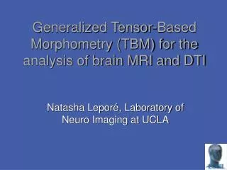
34. Fractional and geodesic anisotropy • In diffusion tensor imaging, “level of directionality” often of interest, e.g. relative and fractional anisotropy • The distance metric on tensors allows a more rigorous definition of this • Anisotropy is measured by the distance between the tensor and its nearest isotropic counterpart • Euclidean distance gives FA • Geodesic Anisotropy uses Riemannian metric • GA = ||H – I tr(H)/2||F

35. tanh(GA)

36. Other measures • Jacobian is gradient of the transformation field • Are div(u) or curl(u) of interest? • First, note contained in J • div(u) = tr(du/dx) = tr(J – I) • curl(u) has same elements as skew-sym J – J’ • div(u) AKA “volume dilatation” • Proposed as part of Chung et al’s “unified” approach

37. Left: log|J| Right: curl(u) Left: div(u) Right: GA

38. Longitudinal TBM • Registration within-subject typically performed first • Inter-subject spatial normalisation follows • For scalar Jacobian determinant can simply resample • More complicated for vector or tensor fields… • Related problem in Diffusion Tensor Imaging • Except there microscopic, here macroscopic

39. a Source Reference b c d • Macroscopic transformation of anatomy, according to image registration • Microscopic properties of water diffusion preserved • Macroscopic compression assumed to represent shorter tracts rather than shorter diffusion scale; hence smaller number of same shape ellipses • Orientation of ellipse transformed according to anatomical transformation, e.g. preserving principle direction of diffusion (PPD) [Alexander et al. 2001]. Continuity of fibre tracts should be preserved.

40. Source A Source B Reference The finite strain reorientation fails to reorient deformation vectors for the changes that occur in anisotropic scaling and/or shearing.

41. s1 c b r1 s0 d a r0 Time 0 Time 1 Source Reference Serial deformation is also macroscopic, and hence transformation in reference space is conjugate to that in source space; compression of source onto reference also compresses longitudinal change.

42. Spatial smoothing • Intra-subject registration over time highly accurate • Inter-subject spatial normalisation much less precise • Spatial smoothing required • Different methods have been developed to reduce the danger of expansion and contraction cancelling out • E.g. VBM, VCM • More work is needed, especially for multivariate TBM

43. Statistical analysis • Similar to VBM, TBM performs voxel-wise tests • Interpretable spatial pattern of significant findings • While VBM and determinant-based TBM are mass-univariate, strain tensors require multivariate statistics • Random field theory not yet well established for Wilks’ L • Assumptions of normality may be more questionable • Estimation of covariance matrices may be unreliable • Non-parametric permutation testing is appealing

44. Assumptions Gaussian error, … Increase in variance due to restrictions ~ F Properties of random field => Pr(max>crit|H0) Assumptions Exchangeable under null Arbitrary statistic Including multivariate Resampling-based distribution of max(stat) => Pr(max>crit|H0) Parametric stats vs. Resampling-based 95th percentile

45. Permutation testing • Track permutations’ image-wise maxima • p-values corrected for Family-Wise (“image-wise”) Error • Empirical null distr. shouldn’t include “active” voxels • Track secondary (etc) maxima and locations • allows more sensitive step-down procedure • Belmonte and Yurgelun-Todd (2001) IEEE TMI 20:243-8 • Computationally intensive • But amenable to parallel implementation

46. Results • 36 probable Alzheimer’s Disease patients • 20 age- and gender-matched control subjects • Baseline and 12 month repeat scans • Standard clinical T1-weighted images • Between- then within-subject registration • 8mm FWHM Gaussian smoothing

47. s(log(det)) 1(1) s:smooth’d s(displ) 3(6) GA(s(H)) 1(1) eig(s(H)) 3(6) s(H) 6(21) s(J) 9(45) As left, butabs(log(p)) for p < 0.05

48. Log-Euc analysis of U, colour-coded by tr(sm(H))

49. det 2 LE 2 det LE 3 2 2 J FDR FWE

50. 2 div disp 3 2 2 curl Some evidence for complementarityof the different measures