Download

1 / 54
540 likes | 821 Vues
BIOL 3300 Vertebrate Zoology: Ectotherms - Herpetology. http://www.amphibian.com.au/. What is Biogeography ?. A study of past and present animal distributions . Example Biogeographical Questions. Why similar distribution of cryptobranchids AND alligators?

E N D
BIOL 3300 Vertebrate Zoology: Ectotherms - Herpetology http://www.amphibian.com.au/
What is Biogeography? A study of past and present animal distributions
Example Biogeographical Questions • Why similar distribution of cryptobranchids AND alligators? • When did Galapagos lizards arrive? • Why vipers & elapids on Africa but not Madagascar? • How did continental movement during Mesozoic and Cenozoic affect diversity?
What data are needed? Biotic data such as… Geological data such as… • Details to follow…
How do you explain disjunct? There are 2 mechanisms for explaining disjunct populations/distributions. 1) 2)
How do you explain disjunct? Bushmasters (Lachesis sp.) are AWESOME snakes…
How do you explain Bushmaster distribution? http://www.usavri.org/Roy%20CR%202009.html http://animaldiversity.ummz.umich.edu
How do you explain Bushmaster distribution? http://www.usavri.org/Roy%20CR%202009.html http://animaldiversity.ummz.umich.edu
How have continents changed? http://www.youtube.com/watch?v=jOzh5YuLVb4
How do you explain the high biodiversity of Central America? • V0 ~ N. & S. Americaseparate(_______________) • D1 ~ ________________
How do you explain the high biodiversity of Central America?
How do you explain the high biodiversity of Central America? • V0 ~ N. & S. Americaseparate (Pangaea) • D1~ Proto Antilles • V1~ N. & S. America separate(___________________)
How do you explain the high biodiversity of Central America?
How do you explain the high biodiversity of Central America? • V0 ~ N. & S. Americaseparate (Pangaea) • D1~ Proto Antilles • V1~ N. & S. America separate(Proto Antilles leave) • D2 ~ ______ (move S.) • V2 ~ _________ • D3 ~ _______________ • V3 ~ _______________
How do you explain the high biodiversity of Central America? • Mountains and areas of high diversity….
How do you explain the high biodiversity of Central America? • V0 ~ N. & S. Americaseparate (Pangaea) • D1~ Proto Antilles • V1~ N. & S. America separate(Proto Antilles leave) • D2 ~ Cooling (move S.) • V2 ~ Desertification • D3 ~ Mountain ranges • V3 ~ Mountain ranges • D4 ~ __________________
How do you explain the high biodiversity of Central America?
How do you explain the high biodiversity of Central America?
Why the high montanediversity? • Mountains and areas of high diversity…. • Can you get too high?
What about North America? • Garter snakes (Thamnophis sp.) are an interesting example….
How is it that some of the fauna of the Galapagos Islands are younger than the island?
Figure 13.1 Diagrammatic reconstruction of the history of continental drift.
Figure 13.2 Graphic depicting two very different approaches to understanding global patterns of species richness. The circle represents the globe, and shades of color represent latitudinal zones with the latitude zero across the center. On the left, black points represent individual species, and clearly the number of species is correlated with latitude; tropical habitats have more species than temperate habitats. Explanations for higher diversity in tropical regions center on correlations between numbers of species and environmental variables such as temperature and moisture. On the right, evolutionary relationships of species are shown (lines) with a hypothetical monophyletic clade represented. This graphic stresses a history of diversification indicating that more clades originated in the tropics, and because of niche conservatism, few clades were able to evolve ecological traits allowing them to disperse to temperate climates. Adapted from Wiens and Donoghue, 2004.
Figure 13.3 Graphical model showing effects of niche conservatism and niche evolution on faunas in different regions of the world. Colored circles represent different clades. Two clades (blue and green) have retained ancestral niche characteristics and have distributions restricted to tropical and subtropical environments. A third clade (black) has evolved tolerance to lower temperatures and lower precipitation and dispersed, no longer occurring in tropical regions and thus showing niche evolution. Adapted from Wiens and Donoghue, 2004.
Figure 13.4 Temperature isotherms and the northern and southern limits of frog (30 species), salamander (26 species), and lizard (16 species) distributions in eastern North America (Piedmont and Coastal Plain). Isotherms are mean annual temperature (°F); the integers in each zone are number of species with ranges terminating in the interval (northern–southern termini). Isotherms from USDA, 1941; distributional data from Conant and Collins, 1991.
Figure 13.5 Geographic variation in clutch size among populations of the snapping turtle (Chelydra serpentina) in North America. Integers indicate mean clutch size at specific locality. Data from Fitch, 1985, and Iverson et al., 1997.
Figure 13.7 Graphical model showing the difference between vicariance and vicariance with a single dispersal event in the construction of area cladograms. At time 1 (T1) the ancestor lives on a single large continent. By time 2, continents have separated, creating the first vicariant event, and additional speciation has occurred on the continent on the right. By time 3, four continents exist. On the left, no dispersal has taken place, and additional speciation events have occurred on continents 1, 3, and 4. On the right, speciation has also occurred on continents 1, 3, and 4, but one of the species on continent 3 has dispersed to continent 2 where, over time, that species has differentiated. Thus the species on continent 2 has one of the species from continent 3 as its closest relative (sister taxon). Cladograms at the top show phylogenetic relationships between the species under each scenario. Numbers across the top refer to present distribution of species on the four continents. By comparing a dated phylogeny with independently derived dates of vicariant events (in this case, continental splitting), it is possible to falsify a vicariance hypothesis. The phylogeny on the left supports a vicariance hypothesis, and the one on the right falsifies it for the species on continent 2, leaving dispersal as the only viable hypothesis for the origin of that species on continent 2. Although our example uses continents, other barriers (mountains, rivers, ecological transitions) can result in vicariance. Adapted in part from Futuyuma, 1998.
Figure 13.8 Comparison of phylogenetic relationships of chelid turtles and their distributions to the tectonics of southern continents. Unfortunately, the most recent cladogram (far right) fails to falsify either of the earlier hypotheses because Chelodina, South American chelids, and remaining Australian chelids form an unresolved polytomy. Cladograms adapted from Gaffney, 1977; Seddon et al., 1997; and Georges et al., 1998.
Figure 13.9 Although diversification of lizards in the Anolis nitens (formerly A. chrysolepis) complex has been used to support the Vanishing Refuge Theory of Amazonian diversity, molecular analysis of the group clearly shows that diversification took place much earlier. Although the described subspecies are each others' closest relatives, a deep split in haplotypes from the north (Roraima state in Brazil and Ecuador) and the south (Amazonas and Acre States in Brazil) and relatively deep splits in more recent clades placed their origins before the existence of proposed refuges. The A. nitens clade, at minimum, is > 15 million years old. Left, maximum parsimony bootstrap tree; right, maximum-likelihood tree. Adapted from Glor et al., 2001.
Figure 13.10 Phylogenetic relationships of Amazonian sphaerodactyline geckos. Based on gene sequence data, major divergences occurred during the Miocene–Pliocene, much before the Pleistocene, when Amazon refuges existed. Adapted from Gamble et al., 2008.
Figure 13.11 The frog Physalaemus petersi is ideal for testing biogeographic hypotheses on origin of diversity in the Amazon River basin because it occurs across an area divided by large rivers (Riverine Hypothesis) and where an elevational gradient exists associated with the Andes (Elevational Gradient Hypothesis). The dotted outline shows the approximate distribution of P. petersi (which extends farther to the east than shown), and the dashed lines show the locations of the Guianan (upper) and Brazilian (lower) Shields. Adapted from Funk et al., 2007.
Figure 13.12 Geographic ranges of major clades of Physalaemus petersi based on haplotype divergences. Numbers indicate average percent corrected sequence divergence. Adapted from Funk et al., 2007.
Figure 13.13 History of diversification of modern amphibians. (A) Phylogeny of modern amphibians with geological timescale across the top. (B) Net diversification rates for amphibian clades. Clade numbers refer to those in (A). Net diversification rates (d – b, where b = speciation rate and d is extinction rate) per clade are shown under the lowest possible relative extinction rate (red, d:b = 0) and an extremely high possible rate (blue, d:b = 0.95). (C) Comparison of proportion diversity of extant amphibian clades in the Late Cretaceous (left) and now (right). Adapted from Roelants et al., 2007.
Figure 13.14 History of global patterns of amphibian net diversification. (A) Rate through time (RTT) plot derived from the time tree (Fig. 13.13) compared with models varying in relative extinction rates from 0 to 0.95. (B) RTT plot of net diversification rates estimated under low extinction rates (red, d:b = 0) and high extinction rates (blue, d:b = 0.95) for successive 20-million-year intervals (280–100 mybp) and 10 million year intervals (100–20 mybp). Circles and asterisks indicate estimates that differ significantly from those expected under low extinction rates (d:b = 0) and high extinction rates (d:b = 0.95), respectively. (C) Amphibian net extinction rates (blue) compared with amniote family origination (green) and extinction (red) rates based on the fossil record. Note that the amphibian data (blue) are represented on a log scale, and thus differences are even more dramatic than shown. Adapted from Roelants et al., 2007.
Figure 13.15 Divergences that most affected global distribution of Microhylidae and Natanura occurred in the Cretaceous. (A) Molecular time tree phylogeny showing divergence patterns. (B) Horizontal colored bars and lines at interval nodes (standard deviation and 95% credibility intervals) indicate vicariance events as follows: orange: Australia <–> Indo-Madagascar; yellow: Africa <–> South America; blue: Africa <–> Indo-Madagascar; purple: Madagascar <–> India (Seychelles); green: South America–Antarctica <–> Indo-Madagascar (with the Kerguelen Plateau involved). (B) Gondwana in the Late Cretaceous. Abbreviations: AF = Africa, MA = Madagascar, In = India, EU = Eurasia, SA = South America, AN = Antarctica, AU = Australia–New Guinea, KP = Kerguelen Plateau. Adapted from Van Bocxlaer et al., 2006.
Figure 13.16 Biogeographic history of ranoid evolution. Dashed branches are lineages of uncertain phylogenetic position. Colored bars across the top of the phylogeny indicate age of ranoid fossils from their respective continents: (1) undetermined ranoids from the Cenomanian of Africa, (2) Ranidae from the Maastrichtian of India, (3) Raninae from the Late Eocene of Europe, and (4) Raninae from the Miocene of North America. Gray shading indicates an apparent lack of dispersal between Africa and other biogeographic units (between nodes 6 and 17) for about 70 million years. The K–T (Cretaceous–Tertiary) boundary is indicated by the vertical dashed line. Asterisks indicate calibration points. Adapted from Bossuyt et al., 2006.
Figure 13.17 Dated phylogeny of ranoid frogs centering on the phylogenetic position of four families endemic to the Western Ghats of India and hills of Sri Lanka, the Ranixalinae, Micrixalinae, Lankanectinae, and Nyctibatrachinae. The phylogeny demonstrates that these clades are outside (sister to) other ranoids. Molecular dating places the origin of the clades containing these four subfamilies in the Cretaceous. Adapted from Roelants et al., 2004.
Figure 13.18 The recently described frog Nasikabatrachus sahyadrensis is among the oldest of the Neobatrachia and ties the fauna of the Seychelles to the fauna of India. Its ancestors must have been present on the Indo-Madagascan fragment of eastern Gondwana during Middle–Late Jurassic or Early Cretaceous. Photograph by S. D. Biju.
Figure 13.19 Early diversification of the Bufonidae occurred near the end of the Upper Cretaceous, failing to confirm a Gondwana origin of the family. Diversification into modern genera occurred later, during the mid-Paleogene. Horizontal bars and shaded rectangles indicate 95% credibility intervals of estimates of divergence times. Colors indicate geographical distributions of each lineage. Adapted from Pramuk et al., 2008.
Figure 13.20 These maps illustrate the key geological events associated with diversification in the Bufonidae. (A) Bufonids originated in South America about 88 mybp, after the breakup of Gondwana. At some point, bufonids dispersed into the Old World and diversified into the Eurasian and African clades, likely across Beringia. (B) Approximately 43 mybp, during the Eocene, bufonids dispersed back into the New World. Although at least three possible routes existed (Berengia, DeGeer, and Thulean land bridges), the Thulean land bridge is most likely because it provided a much more mild climatic regime. Adapted from Pramuk et al., 2008.
Figure 13.21 Phylogenetic relationships of eleutherodactyline frogs showing geographical distribution for each clade. Adapted from Heinicke et al., 2007.
Figure 13.22 The origins of Middle American and Caribbean clades of eleutherodactyline frogs can be modeled based on the timing of divergences. (A) Dispersal over water from their South American origin probably occurred during the Middle Eocene (49-37 mybp), resulting in the formation of the Middle American clade (MAC) and the Caribbean clade (CC). (B) Higher sea levels led to isolation of a western Caribbean clade (WCC) on Cuba and an eastern Caribbean clade on Hispaniola and Puerto Rico during the Early Oligocene (approximately 30 mybp). (C) Dispersal from Cuba to the mainland led to the radiation of the subgenus Syrrhopus in southern North America during the Early Miocene (approximately 20 mybp). Concurrently, members of the ECC and South American clade (SAC) colonized the Lesser Antilles. (D) The closing of the Isthmus of Panama during the Pliocene (approximately 3 mybp) resulted in overland dispersal of MAC species to South America and SAC species to Middle America. Adapted from Heinicke et al., 2007.
Figure 13.23 The first major divergence event in the history of caecilians occurred on Gondwana approximately 178 mybp with several other Gondwana divergences. This deep divergence accounts for the presence of caecilians on most southern continents today. However, an added twist is the much more recent dispersal (40-53 mybp) of members of the Ichthyophiidae into Southeast Asia. Adapted from Pough et al., 2003, and Wilkinson et al., 2002b.
Figure 13.24 Divergence of African caecilians cannot be tied to a single biogeographical event. (A) Left, phylogeny based on 12S and 16S gene sequences; right, uncorrected lognormal molecular clock showing divergence times. (B through G) West (C, E, G) and East (B, D, F) African caecilians. (H) Map of Africa showing current non-overlapping distributions of West and East African caecilians. Adapted from Loader et al., 2007.
Figure 13.25 Although it has been assumed that small fossorial amphibians and reptiles would not be able to disperse across oceans, it appears that amphisbaenians have done just that. Based on the dated phylogeny and the position of landmasses at the time, the only supportable hypothesis for dispersal of Amphisbaenidae ancestors to the New World is transatlantic during the Eocene (arrow 1, upper left). The most likely hypothesis for dispersal of cadeids is transatlantic during the Eocene (solid arrow 2, upper left), although a complex terrestrial dispersal cannot be ruled out (dashed arrow 2, upper left). Adapted from Vidal et al., 2008.
Figure 13.26 Subaerial (surface) connections between Madagascar and Antarctica likely existed approximately 90 mybp. Dark shading indicates submerged areas. Mad = Madagascar, KP = Kerguelen Plateau, GR = Gunnerus Ridge, and EB = Enderby Basin. Adapted from Noonen and Chippindale, 2006.