Scientific Visualization using VTK
Scientific Visualization using VTK. Robert Putnam putnam@bu.edu. Scientific Visualization with VTK – Fall 2010. Outline. Introduction VTK overview VTK data geometry/topology Case study Interactive session. Scientific Visualization with VTK – Fall 2010. Introduction.


Scientific Visualization using VTK
E N D
Presentation Transcript
Scientific Visualization using VTK Robert Putnam putnam@bu.edu Scientific Visualization with VTK – Fall 2010
Outline • Introduction • VTK overview • VTK data geometry/topology • Case study • Interactive session Scientific Visualization with VTK – Fall 2010
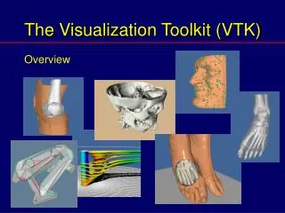
Introduction • Visualization: converting raw data to a form that is viewable and understandable to humans. • Scientific visualization: specifically concerned with data that has a well-defined representation in 2D or 3D space (e.g., from simulation mesh or scanner). *Adaptedfrom The ParaView Tutorial, Moreland Scientific Visualization with VTK – Fall 2010
VTK Visualization Toolkit • Open source • Set of object-oriented class libraries for visualization and data analysis • Several language interfaces • C++ • Tcl • Java • Python • Portable (MS Windows, Linux, OSX) • Active developer community • Good documentation available, free and otherwise • Professional support services available from Kitware Scientific Visualization with VTK – Fall 2010
Generic visualization pipeline Source(s) Filters(s) Output - - - - - - - - - - - - - - - - - - - - - data/geometry/topology graphics Scientific Visualization with VTK – Fall 2010
VTK terminology/model Source Filter Mapper Renderer - - - - - - - - - - - - - - - - - - - - - data/geometry/topology graphics Scientific Visualization with VTK – Fall 2010
VTK terminology/model “Scene" Lights, Camera Actor Source/ Reader Filter Mapper Renderer - - - - - - - - - - - - - - - - - - - - - DataObject ProcessObject RenderWindow graphics data/geometry/topology Scientific Visualization with VTK – Fall 2010
Reader Filter Mapper Actor RenderWindow Renderer Pipeline -> Sample Code vtkStructuredGridReader reader reader SetFileName "density.vtk" reader Update vtkContourFilter iso iso SetInputConnection [reader GetOutputPort] iso SetValue 0 .26 vtkPolyDataMapper isoMapper isoMapper SetInputConnection [iso GetOutputPort] vtkActor isoActor isoActor SetMapper isoMapper vtkRenderer ren1 ren1 AddActor isoActor vtkRenderWindow renWin renWin AddRenderer ren1 renWin SetSize 500 500 renWin Render Scientific Visualization with VTK – Fall 2010
TCL v. C++ • TCL • C++ vtkStructuredGridReader reader reader SetFileName "density.vtk" reader Update vtkContourFilter iso iso SetInputConnection [reader GetOutputPort] iso SetValue 0 .26 vtkStructuredGridReader *reader = vtkStructuredGridReader::New(); reader->SetFileName("density.vtk"); reader->Update(); vtkContourFilter *iso = vtkCountourFilter::New(); iso->SetInputConnection(reader->GetOutputPort()); iso->SetValue(0, .26); Scientific Visualization with VTK – Fall 2010
Coding tip of the day! • Google “VTK class list”, or • Go to: http://www.vtk.org/doc/nightly/html/annotated.html Scientific Visualization with VTK – Fall 2010
VTK – Geometry v. Topology • Geometry of a dataset ~= points 0,1 1,1 2,1 3,1 0,0 1,0 2,0 3,0 • Topology ~= connections among points, which define cells • So, what’s the topology here? Scientific Visualization with VTK – Fall 2010
VTK – Geometry v. Topology 0,1 1,1 2,1 3,1 0,0 1,0 2,0 3,0 Scientific Visualization with VTK – Fall 2010
VTK – Geometry v. Topology 0,1 1,1 2,1 3,1 0,0 1,0 2,0 3,0 or 0,1 1,1 2,1 3,1 0,0 1,0 2,0 3,0 Scientific Visualization with VTK – Fall 2010
VTK – Geometry v. Topology or 0,1 1,1 2,1 3,1 0,1 1,1 2,1 3,1 0,0 1,0 2,0 3,0 0,0 1,0 2,0 3,0 or 0,1 1,1 2,1 3,1 0,0 1,0 2,0 3,0 Scientific Visualization with VTK – Fall 2010
VTK – Geometry v. Topology or 0,1 1,1 2,1 3,1 0,1 1,1 2,1 3,1 0,0 1,0 2,0 3,0 0,0 1,0 2,0 3,0 or or 0,1 1,1 2,1 3,1 0,1 1,1 2,1 3,1 0,0 1,0 2,0 3,0 0,0 1,0 2,0 3,0 Scientific Visualization with VTK – Fall 2010
Geometry/Topology Structure • Structure may be regular or irregular • Regular (structured) • need to store only beginning position, spacing, number of points • smaller memory footprint per cell (topology can be generated on the fly) • examples: image data, rectilinear grid, structured grid • Irregular (unstructured) • information can be represented more densely where it changes quickly • higher memory footprint (topology must be explicitly written) but more freedom • examples: polygonal data, unstructured grid Scientific Visualization with VTK – Fall 2010
Characteristics of Data • Data is organized into datasets for visualization • Datasets consist of two pieces • organizing structure • points (geometry) • cells (topology) • data attributes associated with the structure • File format derived from organizing structure • Data is discrete • Interpolation functions generate data values in between known points Scientific Visualization with VTK – Fall 2010
Structured Points (Image Data) • regular in both topology and geometry • examples: lines, pixels, voxels • applications: imaging CT, MRI • Rectilinear Grid • regular topology but geometry only partially regular • examples: pixels, voxels • Structured Grid (Curvilinear) • regular topology and irregular geometry • examples: quadrilaterals, hexahedron • applications: fluid flow, heat transfer Examples of Dataset Types Scientific Visualization with VTK – Fall 2010
Examples of Dataset Types (cont) • Polygonal Data • irregular in both topology and geometry • examples: vertices, polyvertices, lines, polylines, polygons, triangle strips • Unstructured Grid • irregular in both topology and geometry • examples: any combination of cells • applications: finite element analysis, structural design, vibration Scientific Visualization with VTK – Fall 2010
Examples of Cell Types Scientific Visualization with VTK – Fall 2010
Data Attributes • Data attributes associated with the organizing structure • Scalars • single valued • examples: temperature, pressure, density, elevation • Vectors • magnitude and direction • examples: velocity, momentum • Normals • direction vectors (magnitude of 1) used for shading • Texture Coordinates • used to map a point in Cartesian space into 1, 2, or 3D texture space • used for texture mapping • Tensors • 3x3 only • examples: stress, strain Scientific Visualization with VTK – Fall 2010
File Format – Structured Points Editor structured-points.vtk: # vtk DataFile Version 3.0 first dataset ASCII DATASET STRUCTURED_POINTS DIMENSIONS 3 4 5 ORIGIN 0 0 0 SPACING 1 1 2 POINT_DATA 60 SCALARS temp-point float LOOKUP_TABLE default 0 0 0 1 1 1 1 1 1 0 0 0 0 0 0 1 1 1 1 1 1 0 0 0 0 0 0 1 1 1 1 1 1 0 0 0 0 0 0 1 1 1 1 1 1 0 0 0 0 0 0 1 1 1 1 1 1 0 0 0 Scientific Visualization with VTK – Fall 2010
File Format – Structured Points Editor structured-points.vtk: # vtk DataFile Version 3.0 first dataset ASCII DATASET STRUCTURED_POINTS DIMENSIONS 3 4 5 ORIGIN 0 0 0 SPACING 1 1 2 POINT_DATA 60 SCALARS temp-point float LOOKUP_TABLE default 0 0 0 1 1 1 1 1 1 0 0 0 0 0 0 1 1 1 1 1 1 0 0 0 0 0 0 1 1 1 1 1 1 0 0 0 0 0 0 1 1 1 1 1 1 0 0 0 0 0 0 1 1 1 1 1 1 0 0 0 Scientific Visualization with VTK – Fall 2010
File Format – Structured Points Editor structured-points2.vtk: # vtk DataFile Version 3.0 first dataset ASCII DATASET STRUCTURED_POINTS DIMENSIONS 3 4 5 ORIGIN 0 0 0 SPACING 1 1 2 CELL_DATA 24 SCALARS temp-cell float LOOKUP_TABLE default 0 0 1 1 0 0 0 0 1 1 0 0 0 0 1 1 0 0 0 0 1 1 0 0 Scientific Visualization with VTK – Fall 2010
File Format – Structured Points Editor structured-points2.vtk: # vtk DataFile Version 3.0 first dataset ASCII DATASET STRUCTURED_POINTS DIMENSIONS 3 4 5 ORIGIN 0 0 0 SPACING 1 1 2 CELL_DATA 24 SCALARS temp-cell float LOOKUP_TABLE default 0 0 1 1 0 0 0 0 1 1 0 0 0 0 1 1 0 0 0 0 1 1 0 0 Scientific Visualization with VTK – Fall 2010
Structured Points – Tcl code Editor structured-points.tcl: vtkStructuredPointsReader reader reader SetFileName "structured-points.vtk" reader Update vtkLookupTable lut lut SetNumberOfColors 2 lut SetTableValue 0 0.0 0.0 1.0 1 lut SetTableValue 1 1.0 0.0 0.0 1 vtkDataSetMapper mapper mapper SetInputConnection [reader GetOutputPort] mapper SetLookupTable lut vtkActor actor actor SetMapper mapper [actor GetProperty] EdgeVisibilityOn [actor GetProperty] SetLineWidth 2 Scientific Visualization with VTK – Fall 2010
Structured Points – Tcl code (cont.) Editor structured-points.tcl: vtkRenderer ren1 ren1 AddActor actor ren1 SetBackground 0.5 0.5 0.5 vtkRenderWindow renWin renWin AddRenderer ren1 renWin SetSize 500 500 vtkRenderWindowInteractor iren iren SetRenderWindow renWin iren Initialize wm withdraw . Scientific Visualization with VTK – Fall 2010
Work flow – Case Study • BU Space Physics simulation • Meteor trails in the ionosphere • Data wrangling: • Consolidate datafiles (from parallel code), create single binary datafile • Add VTK header: # vtk DataFile Version 3.0 output of reassemble.c BINARY DATASET STRUCTURED_POINTS ORIGIN 0.0 0.0 0.0 SPACING 1.0 1.0 1.0 DIMENSIONS 512 64 128 POINT_DATA 4194304 SCALARS plasma float LOOKUP_TABLE default Scientific Visualization with VTK – Fall 2010
Work flow – Case Study • Use Tcl for fast development/testing: vtkStructuredPointsReader reader reader SetFileName "opp.vtk" reader Update vtkContourFilter iso iso SetInputConnection \ [reader GetOutputPort] iso SetValue 0 0.1 . . . Scientific Visualization with VTK – Fall 2010
Work flow – Case Study • Add gaussian filter : vtkImageGaussianSmooth gaussian gaussian SetInputConnection [reader GetOutputPort] gaussian SetDimensionality 3 gaussian SetRadiusFactor 1 vtkContourFilter iso iso SetInputConnection \ [gaussian GetOutputPort] iso SetValue 0 0.1 . . . Scientific Visualization with VTK – Fall 2010
Work flow – Case Study • Add more isosurfaces : vtkContourFilter iso iso SetInputConnection [gaussian GetOutputPort] iso SetValue 0 1.0 iso SetValue 1 0.5 iso SetValue 2 0.1 Scientific Visualization with VTK – Fall 2010
Work flow – Case Study • Port to C++, add cutplane, transparency : vtkPlane *plane = vtkPlane::New(); plane->SetOrigin(256,2,63.5); plane->SetNormal(0,1,0); vtkCutter *planeCut = vtkCutter::New(); planeCut->SetInputConnection(reader->GetOutputPort()); planeCut->SetCutFunction(plane); Scientific Visualization with VTK – Fall 2010
Work flow – Case Study • Change color map, use script to loop over *.vtk, generate multiple jpegs, read into Adobe Premiere, produce animation: Scientific Visualization with VTK – Fall 2010
VTK – Getting Started - UI Unix Shell: katana:% cd ~/materials katana:% vtk cone2.tcl Scientific Visualization with VTK – Fall 2010
Keyboard shortcuts j – joystick (continuous) mode t – trackball mode c –camera move mode a –actor move mode left mouse – rotate x,y ctrl - left mouse – rotate z middle mouse –pan right mouse –zoom r –reset camera s/w –surface/wireframe u –command window e –exit Scientific Visualization with VTK – Fall 2010
Code – cone2.tcl Editor cone2.tcl: vtkConeSource cone cone SetResolution 100 vtkPolyDataMapper coneMapper coneMapper SetInput [cone GetOutput] vtkActor coneActor coneActor SetMapper coneMapper [coneActor GetProperty] SetColor 1.0 0.0 0.0 vtkRenderer ren1 ren1 SetBackground 0.0 0.0 0.0 ren1 AddActor coneActor vtkRenderWindow renWin renWin SetSize 500 500 renWin AddRenderer ren1 vtkRenderWindowInteractor iren iren SetRenderWindow renWin iren Initialize Scientific Visualization with VTK – Fall 2010
Exercise Editor: cone3.tcl Add coneActor2, and color it green. (Copy coneActor, and make appropriate changes. Remember to add the new actor to the render window [near the end of the “pipeline”].) Optional: to rotate, scale and set the position away from the origin, use the following: coneActor2 RotateZ 90 coneActor2 SetScale 0.5 0.5 0.5 coneActor2 SetPosition -1.0 0.0 0.0 Scientific Visualization with VTK – Fall 2010
Code – Exercise Editor: cone3.tcl . . . vtkActor coneActor2 coneActor2 SetMapper coneMapper [coneActor2 GetProperty] SetColor 0.0 1.0 0.0 coneActor2 RotateZ 90 coneActor2 SetScale 0.5 0.5 0.5 coneActor2 SetPosition -1.0 0.0 0.0 . . . ren1 AddActor coneActor ren1 AddActor coneActor2 . . . Scientific Visualization with VTK – Fall 2010
VTK - Readers • Image and Volume Readers • vtkStructuredPointsReader - read VTK structured points data files • vtkSLCReader - read SLC structured points files • vtkTIFFReader - read files in TIFF format • vtkVolumeReader - read image (volume) files • vtkVolume16Reader - read 16-bit image (volume) files • Structured Grid Readers • vtkStructuredGridReader - read VTK structured grid data files • vtkPLOT3DReader - read structured grid PLOT3D files • Rectilinear Grid Readers • vtkRectilinearGridReader - read VTK rectilinear grid data files • Unstructured Grid Readers • vtkUnstructuredGridReader - read VTK unstructured grid data files Scientific Visualization with VTK – Fall 2010
VTK - Readers • Polygonal Data Readers • vtkPolyDataReader - read VTK polygonal data files • vtkBYUReader - read MOVIE.BYU files • vtkMCubesReader - read binary marching cubes files • vtkOBJReader - read Wavefront (Maya) .obj files • vtkPLYReader - read Stanford University PLY polygonal data files • vtkSTLReader - read stereo-lithography files • vtkUGFacetReader - read EDS Unigraphic facet files • Image and Volume Readers (add’l) • vtkBMPReader - read PC bitmap files • vtkDEMReader - read digital elevation model files • vtkJPEGReader - read JPEG files • vtkImageReader - read various image files • vtkPNMReader - read PNM (ppm, pgm, pbm) files • vtkPNGRReader - read Portable Network Graphic files Scientific Visualization with VTK – Fall 2010
File Format – Structured Grid Editor density.vtk: # vtk DataFile Version 3.0 vtk output ASCII DATASET STRUCTURED_GRID DIMENSIONS 57 33 25 POINTS 47025 float 2.667 -3.77476 23.8329 2.94346 -3.74825 23.6656 3.21986 -3.72175 23.4982 3.50007 -3.70204 23.3738 3.9116 -3.72708 23.5319 4.1656 -3.69529 23.3312 . . . POINT_DATA 47025 SCALARS Density float LOOKUP_TABLE default 0.639897 0.239841 0.252319 0.255393 0.252118 0.246661 0.240134 0.234116 0.229199 0.225886 0.224268 0.224647 0.231496 0.246895 0.26417 0.27585 0.278987 0.274621 . . . VECTORS Momentum float 0 0 0 13.753 -5.32483 -19.964 42.3106 -15.57 -43.0034 64.2447 -13.3958 -46.2281 73.7861 -4.83205 -36.3829 88.3374 6.23797 -22.8846 . . . Scientific Visualization with VTK – Fall 2010
Clipping, Cutting, Subsampling Selection Algorithms - Clipping • can reveal internal details of surface • VTK - vtkClipDataSet - Cutting/Slicing • cutting through a dataset with a surface • VTK - vtkCutter - Subsampling • reduces data size by selecting a subset of the original data • VTK - vtkExtractGrid Scientific Visualization with VTK – Fall 2010
Code – Clipping Editor: clipping.tcl vtkStructuredGridReader reader reader SetFileName “density.vtk” reader Update vtkPlane plane eval plane SetOrigin [[reader GetOutput] GetCenter] plane SetNormal -0.287 0 0.9579 vtkClipDataSet clip clip SetInputConnection [reader GetOutputPort] clip SetClipFunction plane clip InsideOutOn vtkDataSetMapper clipMapper clipMapper SetInputConnection [clip GetOutputPort] eval clipMapper SetScalarRange [[reader GetOutput] GetScalarRange] vtkActor clipActor clipActor SetMapper clipMapper Scientific Visualization with VTK – Fall 2010
Code – Cutplane/Slicing Editor: cutplane.tcl vtkStructuredGridReader reader reader SetFileName “density.vtk” reader Update vtkPlane plane eval plane SetOrigin [[reader GetOutput] GetCenter] plane SetNormal -0.287 0 0.9579 vtkCutter planeCut planeCut SetInputConnection [reader GetOutputPort] planeCut SetCutFunction plane vtkPolyDataMapper cutMapper cutMapper SetInputConnection [planeCut GetOutputPort] eval cutMapper SetScalarRange [[reader GetOutput] GetScalarRange] vtkActor cutActor cutActor SetMapper cutMapper Scientific Visualization with VTK – Fall 2010
Code – ExtractGrid Editor: extract.tcl vtkStructuredGridReader reader reader SetFileName “density.vtk” reader Update vtkExtractGrid extract extract SetInputConnection [reader GetOutputPort] extract SetVOI -1000 1000 -1000 1000 7 10 extract SetSampleRate 1 1 1 extract IncludeBoundaryOn vtkDataSetMapper mapper mapper SetInputConnection [extract GetOutputPort] eval mapper SetScalarRange [[reader GetOutput] GetScalarRange] vtkActor extractActor extractActor mapper Scientific Visualization with VTK – Fall 2010
Color Mapping • Scalar Algorithms • Color Mapping • maps scalar data to colors • implemented by using scalar values as an index into a color lookup table • specify a HSVA (Hue-Saturation-Value-Alpha) ramp and then generate the colors in the table by using linear interpolation into the HSVA space. • VTK • vtkLookupTable • vtkDataSetMapper Scientific Visualization with VTK – Fall 2010
Code – Color Mapping Editor: colormap.numcolors.tcl . . . vtkLookupTable lut lut SetNumberofColors 16 lut SetHueRange 0.0 0.667 lut Build vtkStructuredGridReader reader reader SetFileName “subset.vtk” reader Update vtkDataSetMapper mapper mapper SetInputConnection [reader GetOutputPort] mapper SetLookupTable lut eval mapper SetScalarRange [[reader GetOutput] GetScalarRange] vtkActor actor actor SetMapper mapper . . . Scientific Visualization with VTK – Fall 2010
Exercise * Change the number of colors in colormap * Reverse the Hue Range * Change the Scalar Range mapper SetScalarRange 0.0 0.7 Scientific Visualization with VTK – Fall 2010
Contouring • Scalar Algorithms (cont) • Contouring • construct a boundary between distinct regions, two steps: • explore space to find points near contour • connect points into contour (2D) or surface (3D) • 2D contour map (isoline): • applications: elevation contours from topography, pressure contours (weather maps) from meteorology3D isosurface: • 3D isosurface: • applications: tissue surfaces from tomography, constant pressure or temperature in fluid flow, implicit surfaces from math and CAD • VTK • vtkContourFilter Scientific Visualization with VTK – Fall 2010
Code – Contour (isoline) Editor: contour.single.tcl . . . vtkStructuredGridReader reader reader SetFileName “subset.vtk” reader Update vtkContourFilter contour contour SetInputConnection [reader GetOutputPort] contour SetValue 0 0.26 vtkPolyDataMapper contourMapper contourMapper SetInputConnection [contour GetOutputPort] eval contourMapper SetScalarRange [[reader GetOutput] GetScalarRange] vtkActor contourActor contourActor SetMapper contourMapper . . . Scientific Visualization with VTK – Fall 2010