Exploring Longitudinal Models in Developmental Twin Research: Genetic and Environmental Influences
This document provides a comprehensive overview of longitudinal modeling techniques in developmental twin research, focusing on estimating the genetic (A), common environmental (C), and unique environmental (E) influences on traits over time. It discusses methods such as Cholesky decomposition and latent growth curve modeling, highlighting their advantages and limitations. The guide emphasizes the importance of using multiple observations from the same individuals to improve power in detecting changes in genetic and environmental influences and examines the factors affecting stability versus change throughout development.


Exploring Longitudinal Models in Developmental Twin Research: Genetic and Environmental Influences
E N D
Presentation Transcript
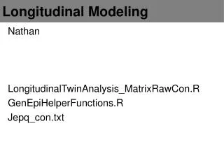
Longitudinal Modeling Nathan & Lindon Template_Developmental_Twin_Continuous_Matrix.R Template_Developmental_Twin_Ordinal_Matrix.R jepq.txt GenEpiHelperFunctions.R
Why run longitudinal models? Map changes in the magnitude of genetic & environmental influence across time ID same versus different genetic or environmental risks across development ID factors driving change versus factors maintaining stability Improve power to detect A, C & E - using multiple observations from the same individual & the cross twin cross trait correlations
Common methods for longitudinal data analyses in genetic epidemiology • Cholesky Decomposition • - Advantages • - Logical: organized such that all factors are constrained to impact later, but not earlier time points • - Requires few assumptions, can predict any pattern of change • - Disadvantages • - Not falsifiable • - No predictions • - Feasible for limited number of measurements • Latent Growth Curve Modeling • Simplex Modeling
Presentation layout Recap common pathway model Latent Growth Models Simplex Models Lindon’s caveat emptor
Phenotype 1 Phenotype 3 Phenotype 2 1 1 1 1 1 1 1 1 1 1 1 1 EC AC CC Common Pathway c11 a11 e11 Common Path f21 f11 f21 AS3 CS3 AS1 CS1 AS2 CS2 ES3 ES1 ES2
Phenotype 1 Phenotype 2 Phenotype 3 1 1 1 1 # Specify a, c & e path coefficients from latent factors A, C & E to Common Pathway mxMatrix( type="Lower", nrow=nf, ncol=nf, free=TRUE, values=.6, name="a" ), # Specify a, c & e path coefficients from residual latent factors As, Cs & Es to observed variables i.e. specifics mxMatrix( type="Diag", nrow=nv, ncol=nv, free=TRUE, values=4, name="as" ), # Specify factor loadings ‘f’ from Common Path to observed variables mxMatrix( type="Full", nrow=nv, ncol=nf, free=TRUE, values=15, name="f" ), # Matrices A, C, & E to compute variance components mxAlgebra( expression = f %&% (a %*% t(a)) + as %*% t(as), name="A" ), AC Common Pathway: Genetic components of variance a11 Common Path ’ as11 as11 ’ = A X as22 + as22 X & f21 as33 as33 f11 f21 as11 as22 as33 As3 As1 As2
# Matrices to store a, c, and e path coefficients for latent phenotype(s) mxMatrix( type="Lower", nrow=nf, ncol=nf, free=TRUE, values=.6, name="a" ), mxMatrix( type="Lower", nrow=nf, ncol=nf, free=TRUE, values=.6, name="c" ), mxMatrix( type="Lower", nrow=nf, ncol=nf, free=TRUE, values=.6, name="e" ), # Matrices to store a, c, and e path coefficients for specific factors mxMatrix( type="Diag", nrow=nv, ncol=nv, free=TRUE, values=4, name="as" ), mxMatrix( type="Diag", nrow=nv, ncol=nv, free=TRUE, values=4, name="cs" ), mxMatrix( type="Diag", nrow=nv, ncol=nv, free=TRUE, values=4, name="es" ), # Matrix f for factor loadings from common pathway to observerd phenotypes mxMatrix( type="Full", nrow=nv, ncol=nf, free=TRUE, values=15, name="f" ), # Matrices A, C, & E to compute variance components mxAlgebra( expression = f %&% (a %*% t(a)) + as %*% t(as), name="A" ), mxAlgebra( expression = f %&% (c %*% t(c)) + cs %*% t(cs), name="C" ), mxAlgebra( expression = f %&% (e %*% t(e)) + es %*% t(es), name="E" ), Common Pathway: Matrix algebra + variance components Within twin (co)variance
# Algebra for expected variance/covariance covMZ <- mxAlgebra( expression= rbind( cbind( A+C+E,A+C), cbind( A+C , A+C+E)), name="expCovMZ" ) covMZ <- mxAlgebra( expression= rbind( cbind( A+C+E , 0.5%x%A+C), cbind(0.5%x%A+C , A+C+E)), name="expCovMZ" ) CP Model: Expected covariance 1 1 / 0.5 Twin 1 Twin 2
Do means & variance components change over time? Are they stable? How to best explain change? Linear, non-linear? One solution == latent growth model Build LGC from scratch Got longitudinal data? Phenotype 1 Time 1 Phenotype 1 Time 2 Phenotype 1 Time 3
AI EI CI 1 1 1 1 1 1 1 1 1 1 1 1 e11 c11 Common Pathway Model a11 B m f31 f11 f21 as33 as11 as22 es22 es11 es33 cs11 cs33 cs22 AS3 CS3 AS1 CS1 AS2 CS2 ES3 ES1 ES2
E1 A1 E2 C2 A2 C1 nf <- 1 nf <- 2 1 1 1 1 1 1 1 1 1 1 1 1 1 1 1 e11 c11 e22 Building a Latent Growth Curve Model a11 a22 c22 B1 B2 m2 m1 f31 f12 f32 f22 f21 f11 Phenotype 1 Time 1 Phenotype 1 Time 2 Phenotype 1 Time 3 as33 as11 as22 es22 es11 es33 cs11 cs33 cs22 AS3 CS3 AS1 CS1 AS2 CS2 ES3 ES1 ES2
C1 E1 A1 A2 C2 E2 e21 c21 a21 nf <- 1 nf <- 2 1 1 1 1 1 1 1 1 1 1 1 1 1 1 1 e11 c11 e22 CP to Latent Growth Curve Model a11 a22 c22 B1 B2 m1 m2 f31 f12 f32 f22 f21 f11 Phenotype 1 Time 1 Phenotype 1 Time 2 Phenotype 1 Time 3 as33 as11 as22 es22 es11 es33 cs11 cs33 cs22 AS3 CS3 AS1 CS1 AS2 CS2 ES3 ES1 ES2
CI Es AI Cs As EI 1 1 1 1 1 1 1 1 1 1 1 1 1 1 1 Intercept: Factor which explains initial variance components (and mean) for all measures. Accounts for the stability over time. Slope: Factor which influences the rate of change in the variance components (and mean) over time. Slope(s) is (are) pre-defined: linear & non linear (quadratic, logistic, gompertz etc) hence factor loading constraints required. e11 c11 e22 Latent Growth Curve Model a11 a22 c22 e21 c21 a21 Bi Bs Intercept Slope im sm 1 0 2 1 1 1 Phenotype 1 Time 1 Phenotype 1 Time 2 Phenotype 1 Time 3 Twin 1 as33 as11 as22 es22 es11 es33 cs11 cs33 cs22 AS3 CS3 AS1 CS1 AS2 CS2 ES3 ES1 ES2
As AI 1 1 1 1 1 Genetic pathway coefficients matrix LGC Model: Within twin genetic components of variance a11 a22 a21 Intercept Slope 1 0 2 Factor loading matrix 1 1 1 Phenotype 1 Time 1 Phenotype 1 Time 2 Phenotype 1 Time 3 Twin 1 as33 as11 as22 aS11 Residual genetic pathway coefficients matrix aS22 AS3 AS1 AS2 aS33
# Matrix for a path coefficients from latent factors to Int’ & Slope latent factors pathAl <- mxMatrix( type="Lower", nrow=nf, ncol=nf, free=TRUE, values=.6, labels=AlLabs, name="al" ) # Matrix for a path coefficients from residuals to observed phenotypes pathAs <- mxMatrix( type="Diag", nrow=nv, ncol=nv, free=TRUE, values=4, labels=AsLabs, name="as" ) # Factor loading matrix of Int & Slop on observed phenotypes pathFl <- mxMatrix( type="Full", nrow=nv, ncol=nf, free=FALSE, values=c(1,1,1,0,1,2), name="fl" ) LGC Model: Specifying variance components in R ’ ’ aS11 aS11 = A aS22 aS22 X + & X aS33 aS33 # Matrix A to compute additive genetic variance components covA <- mxAlgebra( expression=fl %&% (al %*% t(al)) + as %*% t(as), name=“A”)
Simplex Models 1 1 1 1 1 1 I3 I1 I2 i33 i11 i22 LF1 LF3 LF2 lf32 lf21 1 1 1 m2 m1 m3 b1 b3 b2 Phenotype 1 Time 1 Phenotype 1 Time 2 Phenotype 1 Time 3 Twin 1 u33 u11 u22 me me me
Simplex Models Simplex designs model changes in the latent factor structure over time by fitting auto-regressive or Markovian chains Determine how much variation in a trait is caused by stable & enduring effects versus transient effects unique to each time The chief advantage of this model is the ability to partition environmental & genetic variation at each time point into: - genetic & environmental effects unique to each occasion - genetic and environmental effects transmitted from previous time points
Simplex Models 1 1 1 1 1 1 I3 innovations I1 I2 i33 i11 i22 latent factor means latent factors LF1 LF3 LF2 lf32 lf21 means 1 1 1 m3 m2 m1 b3 b2 b1 Phenotype 1 Time 1 Phenotype 1 Time 2 Phenotype 1 Time 3 observed phenotype u33 u11 u22 measurement error me me me
Simplex Models: Within twin genetic variance A1 A2 A3 A1 Transmission pathways A2 A3 Innovation pathways
Simplex Models: Genetic variance A1 A2 A3 A1 Transmission pathways A2 A3 Innovation pathways -1 ’ & - = A * matI <- mxMatrix( type="Iden", nrow=nv, ncol=nv, name="I”) pathAt <- mxMatrix( type="Lower", nrow=nv, ncol=nv, free=tFree, values=ValsA, labels=AtLabs, name="at" ) pathAi <- mxMatrix( type="Diag", nrow=nv, ncol=nv, free=TRUE, values=iVals, labels=AiLabs, name="ai" ) covA <- mxAlgebra( expression=solve( I - at ) %&% ( ai %*% t(ai)), name="A" )
Simplex Models: E variance + measurement error matI <- mxMatrix( type="Iden", nrow=nv, ncol=nv, name="I”) pathEt <- mxMatrix( type="Lower", nrow=nv, ncol=nv, free=tFree, values=tValsE, labels=EtLabs, name="et" ) pathEi <- mxMatrix( type="Diag", nrow=nv, ncol=nv, free=TRUE, values=iVals, labels=EiLabs, name="ei" ) pathMe <- mxMatrix( type="Diag", nrow=nv, ncol=nv, free=TRUE, labels=c("u","u","u"), values=5, name="me" ) covE <- mxAlgebra( expression=solve( I-et ) %&% (ei %*% t(ei))+ (me %*% t(me)), name="E" ) ~ ’ & - * + ’ = E *
Ordinal Data Latent Growth Curve Modeling Es Cs As EI CI AI 1 1 1 1 1 1 1 1 1 1 1 1 1 1 1 e11 c11 e22 a11 a22 c22 e21 c21 a21 Bi Bs Intercept Slope im sm 1 0 2 1 1 1 Phenotype 1 Time 1 Phenotype 1 Time 2 Phenotype 1 Time 3 as33 as11 as22 es22 es11 es33 cs11 cs33 cs22 AS3 CS3 AS1 CS1 AS2 CS2 ES3 ES1 ES2
Intercept Slope Im Sm 1 0 2 1 1 1 Phenotype 1 Time 1 Phenotype 1 Time 2 Phenotype 1 Time 3 Means on observed phenotypes versus means on Intercept & Slope? Bi Bs LGC Model: Estimating means (& sex) in R Twin 1 MeansIS <- mxMatrix( type="Full", nrow=2, ncol=1, free=T, labels=c("Im","Sm"), values=c(5,2), name="LMeans" ) pathB <- mxMatrix( type="Full", nrow=2, ncol=1, free=T, values=c(5,2), labels=c("Bi","Bs"), name="Beta" ) pathFl <- mxMatrix( type="Full", nrow=nv, ncol=nf, free=FALSE, values=c(1,1,1,0,1,2), labels=FlLabs,name="fl" )
Intercept Slope Im Sm 1 0 2 1 1 1 Phenotype 1 Time 1 Phenotype 1 Time 2 Phenotype 1 Time 3 + @ = Expected means for Twin 1 X LGC Model: Means Algebra = X Means1 <- mxAlgebra( expression= ( t((fl %*% ( LMeans - Sex1 %x% Beta )))), name="Mean1") Bi Bs Twin 1