Chapter 5. Ordinary Differential Equation
Chapter 5. Ordinary Differential Equation. 수학과 김찬용 , 컴퓨터학과 김현우 , 장한용. 5.1 The Elementary Theory of Initial-Value Problems. Definition 5.1 f( x , y ) : Lipschitz condition on set D ⊂ R 2 , ∃ L > 0 with , ( t , y 1 ), ( t , y 2 ) ∈ D , L : Lipschitz constant Definition 5.2


Chapter 5. Ordinary Differential Equation
E N D
Presentation Transcript
Chapter 5. Ordinary Differential Equation 수학과 김찬용 , 컴퓨터학과 김현우, 장한용 http://korea.ac.kr
5.1 The Elementary Theory of Initial-Value Problems • Definition 5.1 • f(x,y) : Lipschitz condition on set D⊂R2 , ∃L > 0 with , (t,y1), (t,y2) ∈ D , L : Lipschitz constant • Definition 5.2 • D⊂R2 : convex , (t1,y1), (t2,y2) ∈ D , λ ∈[0,1] ( (1- λ)t1 + λt2 , (1- λ) y1 + λy2 )∈ D i.e. D = { (t , y) | a≤ t≤ b, | y | < ∞ } : convex
5.1 The Elementary Theory of Initial-Value Problems • Definition 5.3 • f(x,y) is defined on a convex set D⊂R2 ∃L > 0 with => f : Lipschitz condition on D with Lipschitz constant L. • Definition 5.4 • , f(x,y) : continuous on D If f satisfies a Lipschitz condition on D, then y′(t) = f(t,y) , a ≤ t ≤ b, y(a) =a has a unique solution y(t) for a ≤ t ≤ b.
5.1 The Elementary Theory of Initial-Value Problems • Definition 5.5 • : well-posed problem if ∃y(t) : unique solution, and ∃ε0 > 0 , ∃k > 0 s.t ∀ε, with ε0 > ε > 0, whenever δ(t) : continuous with |δ(t)| < ε for all t in [a , b] & when |δ0| < ε, dz/dt = z′(t) = f(t,z) + δ(t), a≤ t ≤ b, z(a) = a +δ0 has unique solution z(t) s.t |z(t) - y(t)| < kε for all t in [a , b] • Definition 5.6 • b = { (t,y) | a≤ t ≤ b, |y| < ∞ } f : continuous & Lipschitz condition => dy/dt = f(t,y) , a≤ t ≤ b, y(a) = a : well-posed
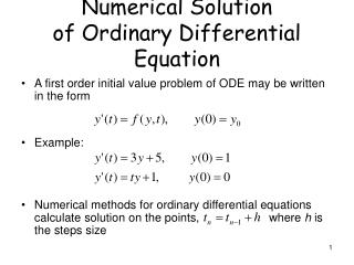
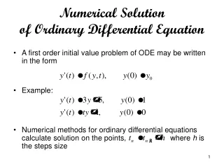
5.2 Euler’s Method • dy/dy = y′(t) = f(t,y) , a ≤ t ≤ b , y(a) = a ti∈[a,b] : mesh points. ti = a + ih , for each i = 0,1,2,… , N ( h= (b-a)/N = ti+1– ti : step size) using Taylor’s Theorem, y(t) ∈ C2[a,b] : unique solution, ∈[a,b] since h= ti+1– ti • Euler’s method :
5.2 Euler’s Method • Lemma 5.7 • ∀x≥ -1 & ∀x > 0, 0≤ (1+x)m ≤ emx • Lemma 5.8 • s,t ∈ R , : then • Theorem 5.9 • f : continuous & Lipschitz condition with L on D &∃M with |y˝(t)| ≤ M,for all t∈[a,b]. Let y(t) : unique solution, Euler’s method =>
5.2 Euler’s Method • Theorem 5.10 • let y(t) : unique solution & u0, u1, … , un : approximation, &|y˝(t)| ≤ M then • : minimal value of E(h)
5.2 High-Order Taylor Methods • Definition 5.11 has local truncation error for each i = 0, 1, … , N -1 Taylor method of order n ω0 = a , ωi = ωi + hT(n)(ti, ωi), for each i = 0, 1, … , N -1 where T(n)(ti, ωi) = f(ti, ωi) + h/2*f ′(ti, ωi) + … + hn-1/n!*f(n-1)(ti, ωi) Note : Euler’s method is Taylor’s method of order one.
5.2 High-Order Taylor Methods • Definition 5.12 using Taylor’s method’s of order n, h: step size. if y ∈ Cn+1[a,b], then the local truncation error is O(hn).
5.4 Runge-Kutta Methods • Definition 5.13 • f(t,y) & all its partial derivatives of order less than or equal to n+1 : continuous on let , ∀ , ∃ ∈(t,t0), ∃ ∈(y,y0) with where : n th Taylor polynomial in two variables.
5.4 Runge-Kutta Methods • ≒ a1T(2)(t,y) + a1b1(t+a1,y+b1) where
5.4 Runge-Kutta Methods => where
5.4 Runge-Kutta Methods • Specific Runge-Kutta method. • Midpoint Method • Modified Euler Method • Heun’s Method
5.4 Runge-Kutta Methods • Runge-Kutta Order Four : for each i = 0, 1, … ,N-1
5.5 Error Control and the Runge-Kutta-Fehlberg Method • (n+1)st – order Taylor method of the form • Producing approximations assume
5.5 Error Control and the Runge-Kutta-Fehlberg Method • Using runge-kutta method with local truncation error of order five, estimate the local error in a runge-kutta method of order four where the coefficient equation are
5.5 Error Control and the Runge-Kutta-Fehlberg Method • The value of q determined at the i th step is used for two purpose • When q<1, to reject the initial choice of h at the i th step and repeat the calculations using qh, and • When q≥1, to accept the computed value at the i th step using the step size h and to change the step size to qh for (i + 1)st step. • n=4 runge-kutta-fehlberg method
5.6 Multistep Methods • Definition 5.14 • m-step multistep method are consistants. when bm = 0 : explicit or open bm≠0 : implicit or closed
5.6 Multistep Methods To begin the derivation of multistep method, Since we can not integrate f(t,y(t)) without knowing y(t) P(t) : interpolating polynomial, (t0, ω0) ….. (ti, ωi) assume
5.6 Multistep Methods • Adams-Bashforth explicit m-step technique Pm-1(t) : backward-difference polynomial, ….. t = ti + sh ,dt = hds , error term
5.6 Multistep Methods • Example three-step Adams-Bashforth technique
5.6 Multistep Methods yi≒ ωi
5.6 Multistep Methods • Definition 5.15 is the (i+1)st step in a multistep method, local truncation error at this step is
5.7 Variable step-size Multistep Method • Adams-Bashforth four-step method ω0, ω1, ... , ωi , μi ∈ (ti-3, ti+1) • Adams-Bashforth three-step method
5.7 Variable step-size Multistep Method new step size qh, generating new approximations As a consequence, we commonly ignore the step-size change when the local truncation error is between ε/10 andε that is when
5.8 Extrapolation Methods assume fixed step size h, y(ti)=y(a+h) let h0 = h/2, use Euler's method with ω0=a , y(a + h0) = y(a+h/2) apply Midpoint method let h = h/4 use Euler's method ω0=a , y(a + h1) = y(a+h/4) with ω1, y(a + 2h1) = y(a+h/2) with ω2 , y(a + 3h1) = y(a+3h/4) with ω3
5.8 Extrapolation Methods approximation
5.9 High-Order Equations and of Differential Equations • m th - order system
5.9 High-Order Equations and of Differential Equations • Definition 5.16 , on satisfy a Lipschitz condition on D, ∃L > 0 with • Definition 5.17 fi(t,u1, ... , um) : continuous on D & satisfy a Lipschitz condition. The system of first-order differential equations, subject to the initial conditions has a unique solution u1(t), ... ,um(t) for a ≤ t ≤ b.
5.9 High-Order Equations and of Differential Equations for each i = 1, 2, ... , m : for each i = 1, 2, ... , m : for each i = 1, 2, ... , m : and then
5.10 Stability • Definition 5.18 • A one-step difference-equation method with local truncation error τi(h) at the i th step is said to be consistent with the differential equation it approximates if • Definition 5.19 • A one-step difference-equation method is said to be convergent with respect to the differential equation it approximates if where yi = y(ti) : exact value of solution of differential equation ωi : approximation obtained from difference method at the with step.
5.10 Stability • Theorem 5.20 is approximated by a one-step difference method in the form ∃h0 > 0, φ(t,w,h) : continuous & satisfies a Lipschitz condition on Then ⅰ) The method is stable; ⅱ) The difference method is convergent if and only if it is consistent, which is equivalent to ⅲ) ∃function and
5.10 Stability • Theorem 5.21 with local truncation error τi+1(h) with local truncation error f(t,y) and fy(t,y) : conditinuous on , fy is bounded then, the local truncation error of the predictor-corrector method is
5.10 Stability • Definition 5.22 • let λ1, λ2, ... , λm : root of the characteristic equation associated with the multistep difference method & if |λi| ≤ 1 , i = 1, 2, ... , m, & all roots with absolute value 1 are simple roots, then the difference method is said to satisfy the root condition.
5.10 Stability • Definition 5.23 ⅰ) Methods the satisfy the root condition and hand λ = 1 as the only root of the characteristic equation of magnitude one are called strongly stable. ⅱ) Methods the satisfy the root condition and have more than one distinct root with magnitude one are called weakly stable. ⅲ) Methods that do not satisfy the root condition are called instable. • Theorem 5.24 • A multistep method of the form where : stable ⇔ root condition moreover, if the difference method is consistant with the difference equation, then the method is stable if it is convergent.
5.11 Stiff Differential Equations : solution, which the transient solution . Euler's method applied to the test equation let h = (b-a) / N , tj = jh , for j = 0, 1, 2, ... , N , so absolute error λ < 0 : (ehλ)j decays to zero as j increases |1+hλ| < 1 : proerty approximation => -2 < hλ < 0 This effectively restricts the step size h for Euler's' method to satisfy h < 2/| λ |
5.11 Stiff Differential Equations ω0 = a + δ0 δ0 : round-off error δ1 : (1+hλ)jδ0 : j th step the round-off error since λ < 0 , the condition for the control of the growth of round-off error is the same as the condition for controlling the absolute error, |1+hλ| < 1, which implies that h < 2/| λ | • Definition 5.24 • The region R of absolute stability for a one-step method is R = { hλ∈C | |Q(hy)| < 1}, and for a multistep method, it is R = { hλ∈C | |bk| < 1, for all zeros bk of Q(z,hy)}.