Download

1 / 42
420 likes | 482 Vues
Explore the concepts of logical reasoning systems, theorem provers, production systems, frame systems, and description logic systems in computer science. Learn about tasks like adding facts to knowledge bases, decision making queries, indexing, and unification algorithms. Discover the basics and syntax of logic programming systems like Prolog.

E N D
Logical reasoning systems • Theorem provers and logic programming languages • Production systems • Frame systems and semantic networks • Description logic systems CS 460, Session 19
Logical reasoning systems • Theorem provers and logic programming languages –Provers: use resolution to prove sentences in full FOL. Languages: use backward chaining on restricted set of FOL constructs. • Production systems –based on implications, with consequents interpreted as action (e.g., insertion & deletion in KB). Based on forward chaining + conflict resolution if several possible actions. • Frame systems and semantic networks –objects as nodes in a graph, nodes organized as taxonomy, links represent binary relations. • Description logic systems –evolved from semantic nets. Reason with object classes & relations among them. CS 460, Session 19
Basic tasks • Add a new fact to KB – TELL • Given KB and new fact, derive facts implied by conjunction of KB and new fact. In forward chaining: part of TELL • Decide if query entailed by KB – ASK • Decide if query explicitly stored in KB – restricted ASK • Remove sentence from KB: distinguish between correcting false sentence, forgetting useless sentence, or updating KB re. change in the world. CS 460, Session 19
Indexing, retrieval & unification • Implementing sentences & terms: define syntax and map sentences onto machine representation. Compound: has operator & arguments. e.g., c = P(x) Q(x) Op[c] = ; Args[c] = [P(x), Q(x)] • FETCH: find sentences in KB that have same structure as query. ASK makes multiple calls to FETCH. • STORE: add each conjunct of sentence to KB. Used by TELL. e.g., implement KB as list of conjuncts TELL(KB, A B) TELL(KB, C D) then KB contains: [A, B, C, D] CS 460, Session 19
Complexity • With previous approach, FETCH takes O(n) time on n-element KB STORE takes O(n) time on n-element KB (if check for duplicates) Faster solution? CS 460, Session 19
Table-based indexing • What are you indexing on? Predicates (relations/functions). Example: CS 460, Session 19
Table-based indexing • Use hash table to avoid looping over entire KB for each TELL or FETCH e.g., if only allowed literals are single letters, use a 26-element array to store their values. • More generally: - convert to Horn form - index table by predicate symbol - for each symbol, store: list of positive literals list of negative literals list of sentences in which predicate is in conclusion list of sentences in which predicate is in premise CS 460, Session 19
Tree-based indexing • Hash table impractical if many clauses for a given predicate symbol • Tree-based indexing (or more generally combined indexing): compute indexing key from predicate and argument symbols Predicate? First arg? CS 460, Session 19
Tree-based indexing Example: Person(age,height,weight,income) Person(30,72,210,45000) Fetch( Person(age,72,210,income)) Fetch(Person(age,height>72,weight<210,income)) CS 460, Session 19
Unification algorithm: Example Understands(mary,x) implies Loves(mary,x) Understands(mary,pete) allows the system to substitute pete for x and make the implication that IF Understands(mary,pete) THEN Loves(mary,pete) CS 460, Session 19
Unification algorithm • Using clever indexing, can reduce number of calls to unification • Still, unification called very often (at basis of modus ponens) => need efficient implementation. • See AIMA p. 303 for example of algorithm with O(n^2) complexity (n being size of expressions being unified). CS 460, Session 19
Logic programming Remember: knowledge engineering vs. programming… CS 460, Session 19
Logic programming systems e.g., Prolog: • Program = sequence of sentences (implicitly conjoined) • All variables implicitly universally quantified • Variables in different sentences considered distinct • Horn clause sentences only (= atomic sentences or sentences with no negated antecedent and atomic consequent) • Terms = constant symbols, variables or functional terms • Queries = conjunctions, disjunctions, variables, functional terms • Instead of negated antecedents, use negation as failure operator: goal NOT P considered proved if system fails to prove P • Syntactically distinct objects refer to distinct objects • Many built-in predicates (arithmetic, I/O, etc) CS 460, Session 19
Prolog systems CS 460, Session 19
Basic syntax of facts, rules and queries <fact> ::= <term> . <rule> ::= <term> :- <term> . <query> ::= <term> . <term> ::= <number> | <atom> | <variable> | <atom> (<terms>) <terms> ::= <term> | <term>, <terms> CS 460, Session 19
A PROLOG Program • A PROLOG program is a set of facts and rules. • A simple program with just facts : parent(alice, jim). parent(jim, tim). parent(jim, dave). parent(jim, sharon). parent(tim, james). parent(tim, thomas). CS 460, Session 19
A PROLOG Program • c.f. a table in a relational database. • Each line is a fact (a.k.a. a tuple or a row). • Each line states that some person X is a parent of some (other) person Y. • In GNU PROLOG the program is kept in an ASCII file. CS 460, Session 19
A PROLOG Query • Now we can ask PROLOG questions : | ?- parent(alice, jim). yes | ?- parent(jim, herbert). no | ?- CS 460, Session 19
A PROLOG Query • Not very exciting. But what about this : | ?- parent(alice, Who). Who = jim yes | ?- • Who is called a logical variable. • PROLOG will set a logical variable to any value which makes the query succeed. CS 460, Session 19
A PROLOG Query II • Sometimes there is more than one correct answer to a query. • PROLOG gives the answers one at a time. To get the next answer type ;. | ?- parent(jim, Who). Who = tim ? ; Who = dave ? ; Who = sharon ? ; yes | ?- NB : The ; do not actually appear on the screen. CS 460, Session 19
A PROLOG Query II | ?- parent(jim, Who). Who = tim ? ; Who = dave ? ; Who = sharon ? ; yes | ?- • After finding that jim was a parent of sharon GNU PROLOG detects that there are no more alternatives for parent and ends the search. NB : The ; do not actually appear on the screen. CS 460, Session 19
conjunction Prolog example CS 460, Session 19
Append • append([], L, L) • append([H| L1], L2, [H| L3]) :- append(L1, L2, L3) • Example join [a, b, c] with [d, e]. • [a, b, c] has the recursive structure [a| [b, c] ]. • Then the rule says: • IF [b,c] appends with [d, e] to form [b, c, d, e] THEN [a|[b, c]] appends with [d,e] to form [a|[b, c, d, e]] • i.e. [a, b, c] [a, b, c, d, e] CS 460, Session 19
Expanding Prolog • Parallelization: OR-parallelism: goal may unify with many different literals and implications in KB AND-parallelism: solve each conjunct in body of an implication in parallel • Compilation: generate built-in theorem prover for different predicates in KB • Optimization: for example through re-ordering e.g., “what is the income of the spouse of the president?” Income(s, i) Married(s, p) Occupation(p, President) faster if re-ordered as: Occupation(p, President) Married(s, p) Income(s, i) CS 460, Session 19
Theorem provers • Differ from logic programming languages in that: - accept full FOL - results independent of form in which KB entered CS 460, Session 19
OTTER • Organized Techniques for Theorem Proving and Effective Research (McCune, 1992) • Set of support (sos): set of clauses defining facts about problem • Each resolution step: resolves member of sos against other axiom • Usable axioms (outside sos): provide background knowledge about domain • Rewrites (or demodulators): define canonical forms into which terms can be simplified. E.g., x+0=x • Control strategy: defined by set of parameters and clauses. E.g., heuristic function to control search, filtering function to eliminate uninteresting subgoals. CS 460, Session 19
OTTER • Operation: resolve elements of sos against usable axioms • Use best-first search: heuristic function measures “weight” of each clause (lighter weight preferred; thus in general weight correlated with size/difficulty) • At each step: move lightest close in sos to usable list, and add to usable list consequences of resolving that close against usable list • Halt: when refutation found or sos empty CS 460, Session 19
Example CS 460, Session 19
Example: Robbins Algebras Are Boolean • The Robbins problem---are all Robbins algebras Boolean?---has been solved: Every Robbins algebra is Boolean. This theorem was proved automatically by EQP, a theorem proving program developed at Argonne National Laboratory CS 460, Session 19
Example: Robbins Algebras Are Boolean Historical Background • In 1933, E. V. Huntington presented the following basis for Boolean algebra: x + y = y + x. [commutativity] (x + y) + z = x + (y + z). [associativity] n(n(x) + y) + n(n(x) + n(y)) = x. [Huntington equation] • Shortly thereafter, Herbert Robbins conjectured that the Huntington equation can be replaced with a simpler one: n(n(x + y) + n(x + n(y))) = x. [Robbins equation] • Robbins and Huntington could not find a proof, and the problem was later studied by Tarski and his students CS 460, Session 19
Given to the system CS 460, Session 19
Forward-chaining production systems • Prolog & other programming languages: rely on backward-chaining (I.e., given a query, find substitutions that satisfy it) • Forward-chaining systems: infer everything that can be inferred from KB each time new sentence is TELL’ed • Appropriate for agent design: as new percepts come in, forward-chaining returns best action CS 460, Session 19
Implementation • One possible approach: use a theorem prover, using resolution to forward-chain over KB • More restricted systems can be more efficient. • Typical components: - KB called “working memory” (positive literals, no variables) - rule memory (set of inference rules in form p1 p2 … act1 act2 … - at each cycle: find rules whose premises satisfied by working memory (match phase) - decide which should be executed (conflict resolution phase) - execute actions of chosen rule (act phase) CS 460, Session 19
Match phase • Unification can do it, but inefficient • Rete algorithm (used in OPS-5 system): example rule memory: A(x) B(x) C(y) add D(x) A(x) B(y) D(x) add E(x) A(x) B(x) E(x) delete A(x) working memory: {A(1), A(2), B(2), B(3), B(4), C(5)} • Build Rete network from rule memory, then pass working memory through it CS 460, Session 19
Rete network D A=D add E A B A=B C add D E A=E delete A C(5) D(2) A(1), A(2) B(2), B(3), B(4) A(2), B(2) Circular nodes: fetches to WM; rectangular nodes: unifications A(x) B(x) C(y) add D(x) A(x) B(y) D(x) add E(x) A(x) B(x) E(x) delete A(x) {A(1), A(2), B(2), B(3), B(4), C(5)} CS 460, Session 19
D A=D Add E A B A=B C Add D E A=E Delete A { A(1), A(2), B(2), B(3), B(4), C(5), Rete match A(x) B(x) C(y) add D(x) A(x) B(y) D(x) add E(x) A(x) B(x) E(x) delete A(x) A(2) D(2) x/2 D(2) E(2) D(2) C(5) y/5 A(1), A(2) B(2),B(3),B(4) A(2) B(2) x/2 E(2) A(2) E(2) x/2 Delete A(2) E(2) } D(2), CS 460, Session 19
Advantages of Rete networks • Share common parts of rules • Eliminate duplication over time (since for most production systems only a few rules change at each time step) CS 460, Session 19
Conflict resolution phase • one strategy: execute all actions for all satisfied rules • or, treat them as suggestions and use conflict resolution to pick one action. • Strategies: - no duplication (do not execute twice same rule on same args) - regency (prefer rules involving recently created WM elements) - specificity (prefer more specific rules) - operation priority (rank actions by priority and pick highest) CS 460, Session 19
Frame systems & semantic networks • Other notation for logic; equivalent to sentence notation • Focus on categories and relations between them (remember ontologies) • e.g., Cats Mammals Subset CS 460, Session 19
Syntax and Semantics Link Type A B A B A B A B A B Semantics A B A B R(A,B) x x A R(x,y) x y x A y B R(x,y) Subset Member R R R CS 460, Session 19
Semantic Network Representation Breath can has Skin Animal can Move Is a Is a Fly can has Fish Wings Bird has Feathers Is a Is a Canary Ostrich is can is cannot Sing Yellow Fly Tall CS 460, Session 19
Subset Member Member R Parent Semantic network link types Link type Semantics Example A B A B Cats Mammals A B A B Bill Cats A B R(A, B) Bill 12 A B x x A R(x, B) Birds 2 A B x y x A y B R(x, y) Birds Birds Subset R Age Legs R CS 460, Session 19