Download
1 / 88
880 likes | 1.06k Vues
Super-Resolution Reconstruction of Images - Static and Dynamic Paradigms. February 2002. Michael Elad* The Scientific Computing and Computational Mathematics Program - Stanford.

E N D
Super-Resolution Reconstruction of Images - Static and Dynamic Paradigms February 2002 Michael Elad* The Scientific Computing and Computational Mathematics Program - Stanford * Joint work with Prof. Arie Feuer – The Technion, Haifa Israel, Prof. Yacob Hel-Or – IDC, Herzelia, Israel, Tamir Sagi - Zapex-Israel.
Static Versus Dynamic Super-Resolution Definitions and Activity Map
Basic Super-Resolution Idea Given: A set of degraded (warped, blurred, decimated, noised) images: Required: Fusion of the measurements into a higher resolution image/s
Static Super-Resolution (SSR) t Low Resolution Measurements Static Super-Resolution Algorithm High Resolution Reconstructed Image
Dynamic Super-Resolution (DSR) Dynamic Super-Resolution Algorithm Low Resolution Measurements t High Resolution Reconstructed Images t
* This table probably does mis-justice to someone - no harm meant Methods which relate also to DSR paradigm. All others deal with SSR. Other Work In this Field
Our Work In this Field M. Elad and A. Feuer, “Restoration of Single Super-Resolution Image From Several Blurred, Noisy and Down-Sampled Measured Images”, the IEEE Trans. on Image Processing, Vol. 6, no. 12, pp. 1646-58, December 1997. M. Elad and A. Feuer, “Super-Resolution Restoration of Continuous Image Sequence - Adaptive Filtering Approach”, the IEEE Trans. on Image Processing, Vol. 8. no. 3, pp. 387-395, March 1999. M. Elad and A. Feuer, “Super-Resolution reconstruction of Continuous Image Sequence”, the IEEE Trans. On Pattern Analysis and Machine Intelligence (PAMI), Vol. 21, no. 9, pp. 817-834, September 1999. M. Elad and Y. Hel-Or, “A Fast Super-Resolution Reconstruction Algorithm for Pure Translational Motion and Common Space Invariant Blur”, Accepted to the IEEE Trans. on Image Processing, March 2001. T. Sagi, A. Feuer and M. Elad, “The Periodic Step Gradient Descent Algorithm - General Analysis and Application to the Super-Resolution Reconstruction Problem”, EUSIPCO 1998. All found in http://sccm.stanford.edu/~elad
Super-Resolution Basics Intuition and Relation to Sampling theorems
For a given band-limited image, the Nyquist sampling theorem states that if a uniform sampling is fine enough (D), perfect reconstruction is possible. D D Simple Example
2D 2D Simple Example Due to our limited camera resolution, we sample using an insufficient 2D grid
2D 2D Simple Example However, we are allowed to take a second picture and so, shifting the camera ‘slightly to the right’ we obtain
Simple Example Similarly, by shifting down we get a third image 2D 2D
Simple Example And finally, by shifting down and to the right we get the fourth image 2D 2D
This is Super-Resolution in its simplest form Simple Example - Conclusion It is trivial to see that interlacing the four images, we get that the desired resolution is obtained, and thus perfect reconstruction is guaranteed.
Uncontrolled Displacements In the previous example we counted on exact movement of the camera by D in each direction. What if the camera displacement is uncontrolled?
Uncontrolled Displacements It turns out that there is a sampling theorem due to Yen (1956) and Papulis (1977) covering this case, guaranteeing perfect reconstruction for periodic uniform sampling if the sampling density is high enough (1 sample per each D-by-D square).
Uncontrolled Rotation/Scale/Disp. In the previous examples we restricted the camera to move horizontally/vertically parallel to the photograph object. What if the camera rotates? Gets closer to the object (zoom)?
There is no sampling theorem covering this case Uncontrolled Rotation/Scale/Disp.
Further Complications Sampling is not a point operation – there is a blur • Motion may include perspective warp, local motion, etc. • Samples may be noisy – any reconstruction process must take that into account.
Static Super-Resolution The creation of a single improved image, from the finite measured sequence of images
SSR - The Model Geometric Warp Blur Decimation Y High- Resolution Image 1 F =I H D D H V V Low- Resolution Images 1 1 1 1 N X Additive Noise Y N F N N N
The Warp As a Linear Operation 0 0 F[j,i]=1 Z X Per every point in X find a matching point in Z
Model Assumptions We assume that the images Yk and the operators Hk, Dk, Fk,& Wk are known to us, and we use them for the recovery of X. Yk – The measured images (noisy, blurry, down-sampled ..) Hk – The blur can be extracted from the camera characteristics Dk – The decimation is dictated by the required resolution ratio Fk – The warp can be estimated using motion estimation Wk – The noise covariance can be extracted from the camera characteristics
A Thumb Rule on Desired Resolution In the noiseless case we have Example: Assume that we have N images of M-by-M pixels, and we would like to produce an image X of size L-by-L. Then – Clearly, this linear system of equations should have more equations than unknowns in order to make it possible to have a unique Least-Squares solution.
The Maximum-Likelihood Approach Geometric Warp Blur Decimation Y High- Resolution Image 1 F =I H V H V D D Low- Resolution Images 1 1 1 N 1 X Additive Noise Y N F N N N ? Which X would be such that when fed to the above system it yields a set Yk closest to the measured images
SSR - ML Reconstruction (LS) Minimize: Thus, require:
SSR - MAP Reconstruction Add a term which penalizes for the solution image quality Possible Prior functions - Examples: 1. - simple spatially adaptive, 2. - M estimator (robust functions), Note: Convex prior guarantees convex programming problem
Iterative Reconstruction Assuming the prior is used For , the matrix R is sparse OPTION: Using the SD algorithm (10-15 iterations are enough)
Image-Based Processing SD* Iteration: All the above operations can be interpreted as operations performed on images. AND THUS There is no actual need to use the Matrix-Vector notations as shown here. This notations is important for the development of the algorithm Back projection Simulated error Weighted edges * Also true for the Conjugate Gradient algorithm
SSR – Simpler Problems Y 1 F =I H V V D D H 1 1 1 1 N X Y N F N N N
SSR – Simpler Problems Using
Example 1 Synthetic case: From a single image create 9 3:1 images this way
Example 1 The higher resolution original The reconstructed result One of the low-resolution images Synthetic case: 9 images, no blur, 1:3 ratio
Example 2 16 images, ratio 1:2, PSF - assumed to be Gaussian with =2.5 Taken from one of the given images Taken from the reconstructed result
Dynamic Super-Resolution Low Quality Movie In – High Quality Movie Out
Dynamic Super-Resolution (DSR) Dynamic Super-Resolution Algorithm Low Resolution Measurements t High Resolution Reconstructed Images t
Modeling the Problem ? Low Resolution Measurements t High Resolution Reconstructed Images t Bypass
DSR – From Model to ML The DSR problem is referred to as a long sequence of SSR problems. Thus, Our model is Using ML approach and this function should be minimized per each t.
Note that (apart from the need to solve the linear set), one has to compute L and Z per each t all over again, and the summations length grow linearly in t. Solving the ML Minimizing amounts to solving the linear set of equations where
Recursive Representation Simplifies to (Using )
Alternative Approach Instead of continuing with the previous model and recursive representation, we adopt a different point of view. The new point of view is based on State-Space modeling of our problems This new model leads to better-understanding of the required algorithmic steps towards an efficient solution. The eventual expressions with the alternative method are exactly the same as the ones shown previously. Bypass
DSR - The Model (1) G(t) X(t) - High-resolution image G(t) - Warp operation V(t) - Sequence innovation assumed The System’s Equation V(t) X(t-1) X(t) Delay
Y(t) - Measured image H(t) - Blur D - Decimation N(t) - additive noise S - Laplacian U(t) - Non-smooth. 0 H(t) S- Laplacian U(t) DSR - The Model (2) The Measurements Equation N(t) Y(t) X(t) D
DSR - The Model (3) These two equations form aSpatio-Temporal Prior forcing spatial smoothness & temporal motion compensated smoothness
DSR - Reconstruction By KF The model is given in a State-Space form The basic idea: 1.Since all the inputs are Gaussians, so is X(t) 2. We know all about X(t) if its two first moments are known - In order to estimate X(t) in time, we need to apply Kalman Filter (KF)
1. We start by knowing the pair 2. Based on we get the Prediction Equations: 3. Based on we get the Update Equations: KF: Mean-Covariance Pair
Information pair is defined by The recursive equations become: Interpolation: Update: Presumably, there is nothing to gain in using the information pair, over the mean-covariance pair KF: Information Pair
1. Experimental results indicate that the information matrix is sparser: 2. We intend to avoid the use of Q(t). Therefore, it is natural to achieve simplifying the equation while approximating Q(t). -1 = Information Pair Is Better !!(for our application)