Advanced Techniques in Image Database Retrieval
380 likes | 410 Vues
Explore advanced methods in searching image databases, including color histograms and shape-based similarity measures. Learn about comparing sources of information and improving retrieval accuracy over time.

Advanced Techniques in Image Database Retrieval
E N D
Presentation Transcript
Lecture 25 Searching Image Databases CSE 6367 – Computer Vision Spring 2010 Vassilis Athitsos University of Texas at Arlington
Image Databases • Photographs.
Image Databases • Art clips.
Video Databases • Movies.
Video Databases • Movies, TV footage, YouTube, …
Retrieval and Indexing • Retrieval: identifying content of interest. • Indexing: preprocessing the data, so as to allow fast retrieval.
Holy Grail: Query by Content • Find pictures of a rocky coast.
Holy Grail: Query by Content • Find pictures of John with trees and snow in the background..
Problem: Knowing the Content • How can computers recognize rocky coasts?
Comparing Sources of Information • Learning to recognize classes of images: • Plus: once they are built, they run by themselves. • Minus: very costly to build. • They require tons of training data, labeled by humans. • Minus: they tend to be very inaccurate in practice. • Accuracy improves year by year… • Minus: they can be very slow.
Comparing Sources of Information • Surrounding text: • Plus: in some cases, readily available. • E.g.: web pages. • Plus: when available, it can be used for free. • Plus: oftentimes pretty accurate. • Minus: in some cases, not available. • E.g.: many photo albums. • Minus: oftentimes pretty inaccurate. • You will never find a picture of Michael Jordan unless the words “Michael Jordan” are nearby.
Comparing Sources of Information • Manual labeling: • Plus: labels anticipate what users would look for. • Improves accuracy. • Minus: in some cases, not available. • E.g.: many photo albums, web pages. • Minus: oftentimes pretty inaccurate. • It is hard to anticipate what keywords a user will employ: • “bike ride in the sunset” vs. “sports activity at the end of the day.”
Similarity-Based Retrieval • Query: an example of what we are looking for. query results
Describing Color • How do we describe the color content of this image? query
Describing Color • How do we describe the color content of this image? • Green and blue. query
Describing Color • How do we describe the color content of this image? • Green and blue. • Green at the bottom, blue at the top. query
Describing Color • How do we describe the color content of this image? • A command the computer can understand: • Find images that are green and blue like this. query
A Color Histogram Example • Choose 100 representative colors (or any other number). • In conventional image formats, 16 million colors. • Create an array (color histogram) of length 100. • For each color: • Count how many pixels in the image are closer to that color than to any other of the 100 colors. • Store result in the array. representative colors query
Comparing Histograms • (x1, x2, …, x100) | x1 - y1| + … + | x100 – y100| • (y1, y2, …, y100) | x1 - z1| + … + | z100 – z100| • (z1, z2, …, z100) query a database image another database image
Expected Results similar images query results
Expected Results similar images query results
Expected Results query Colors do not match well enough
Beyond Color Histograms • Some times, shape information is important.
Shape-Based Similarity Measures • Chamfer Distance. • Shape Context.
Shape Context • Choose r1, r2, …, rk • Choose s = number of sectors. • Create a template consisting of rings and sectors, as shown in the image. • Give a number to each sector of each ring. • For each edge pixel: • Center the template on the pixel. • For each sector of each ring, count the number of edge pixels in that sector. • Result: each point ismapped to ? numbers. source: Wikipedia
Shape Context • Choose r1, r2, …, rb • Choose s = number of sectors. • Create a template consisting of rings and sectors, as shown in the image. • Give a number to each sector of each ring. • For each edge pixel: • Center the template on the pixel. • For each sector of each ring, count the number of edge pixels in that sector. • Result: each point ismapped to sb numbers. source: Wikipedia
Shape Representation • Pick T points from each shape, uniformly sampled. • Extract, for each point, the shape context vector. • Then, each shape is represented as a matrix of size ? source: Wikipedia
Shape Representation • Pick T points from each shape, uniformly sampled. • Extract, for each point, the shape context vector. • Then, each shape is represented as a matrix of size T * k. • T: number of points we pick from each shape. • k = s * b. • s: number of sectors in each ring. • b: number of rings. source: Wikipedia
Shape Matching • Each shape is mapped to a matrix of size T*k. • T: number of points we pick from each shape. • k = s * b. • s: number of sectors in each ring. • b: number of rings. • What is the cost of matching two shapes?
Shape Matching • Each shape is mapped to a matrix of size T*k. • T: number of points we pick from each shape. • k = s * b. • s: number of sectors in each ring. • b: number of rings. • What is the cost of matching two shapes? • Simpler question: what is the cost of matching two shape contexts?
Shape Matching • Each shape is mapped to a matrix of size T*k. • T: number of points we pick from each shape. • k = s * b. • s: number of sectors in each ring. b: number of rings. • What is the cost of matching two shapes? • Simpler question: what is the cost of matching two shape contexts? • One answer: Euclidean or Manhattan distance. • Better answer: chi-square distance. • g(k) and h(k): k-th valuesof the two shape contexts.
Shape Matching • Each shape is mapped to a matrix of size T*k. • T: number of points we pick from each shape. • k = s * b. • s: number of sectors in each ring. b: number of rings. • What is the cost of matching two shapes? • Key problem: we do not know what point in one image corresponds to what point in the other image. • Solution: find optimal 1-1 correspondences. • The cost of each correspondence is the matching cost of the shape contexts of the two corresponding points. • What algorithm can be used here?
Shape Matching • Each shape is mapped to a matrix of size T*k. • T: number of points we pick from each shape. • k = s * b. • s: number of sectors in each ring. b: number of rings. • What is the cost of matching two shapes? • Key problem: we do not know what point in one image corresponds to what point in the other image. • Solution: find optimal 1-1 correspondences. • The cost of each correspondence is the matching cost of the shape contexts of the two corresponding points. • This is a bipartite matching problem. • Solution: Hungarian Algorithm. • Complexity:
Shape Matching • Each shape is mapped to a matrix of size T*k. • T: number of points we pick from each shape. • k = s * b. • s: number of sectors in each ring. b: number of rings. • What is the cost of matching two shapes? • Key problem: we do not know what point in one image corresponds to what point in the other image. • Solution: find optimal 1-1 correspondences. • The cost of each correspondence is the matching cost of the shape contexts of the two corresponding points. • This is a bipartite matching problem. • Solution: Hungarian Algorithm. • Complexity: cubic to the number of points.
Shape Context Distance • Proposed by Belongie et al. (2001). • Error rate: 0.63%, with database of 20,000 images. • Uses bipartite matching (cubic complexity!). • 22 minutes/object, heavily optimized.