
Indoor Scene Segmentation using a Structured Light Sensor
E N D
Presentation Transcript
Indoor Scene Segmentation using a Structured Light Sensor ICCV 2011 Workshop on 3D Representation and Recognition Nathan Silberman andRob Fergus Courant Institute
Overview Indoor Scene Recognition using the Kinect • Introduce new Indoor Scene Depth Dataset • Describe CRF-based model • Explore the use of rgb/depth cues
Motivation • Indoor Scene recognition is hard • Far less texture than outdoor scenes • More geometric structure
Motivation • Indoor Scene recognition is hard • Far less texture than outdoor scenes • More geometric structure • Kinect gives us depth map (and RGB) • Direct access to shape and geometry information
Overview Indoor Scene Recognition using the Kinect • Introduce new Indoor Scene Depth Dataset • Describe CRF-based model • Explore the use of rgb/depth cues
Statistics of the Dataset * Labels obtained via LabelMe
Dataset Examples Living Room RGB Raw Depth Labels
Dataset Examples Living Room RGB Depth* Labels * Bilateral Filtering used to clean up raw depth image
Dataset Examples Bathroom RGB Depth Labels
Dataset Examples Bedroom RGB Depth Labels
Existing Depth Datasets RGB-D Dataset [1] [1] K. Lai, L. Bo, X. Ren, and D. Fox. A Large-Scale Hierarchical Multi-View RGB-D Object Dataset. ICRA 2011 [2] B. Liu, S. Gould and D. Koller. Single Image Depth Estimation from Predicted Semantic Labels. CVPR 2010 Stanford Make3d [2]
Existing Depth Datasets Point Cloud Data [1] B3DO [2] [1] AbhishekAnand, HemaSwethaKoppula, Thorsten Joachims, AshutoshSaxena. Semantic Labeling of 3D Point Clouds for Indoor Scenes. NIPS, 2011 [2] A. Janoch, S. Karayev, Y. Jia, J. T. Barron, M. Fritz, K. Saenko, T. Darrell. A Category-Level 3-D Object Dataset: Putting the Kinect to Work. ICCV Workshop on Consumer Depth Cameras for Computer Vision. 2011
Dataset Freely Available http://cs.nyu.edu/~silberman/nyu_indoor_scenes.html
Overview Indoor Scene Recognition using the Kinect • Introduce new Indoor Scene Depth Dataset • Describe CRF-based model • Explore the use of rgb/depth cues
Segmentation using CRF Model Cost(labels) = Local Terms(labeli) + Spatial Smoothness (label i, label j) • Standard CRF formulation • Optimized via graph cuts • Discrete label set (~12 classes)
Model Cost(labels) = Local Terms(labeli) + Spatial Smoothness (label i, label j) = Appearance(labeli | descriptor i) Location(i)
Model Cost(labels) = Local Terms(labeli) + Spatial Smoothness (label i, label j) = Appearance(labeli | descriptor i) Location(i)
Appearance Term Appearance(labeli | descriptor i) • Several Descriptor Types to choose from: • RGB-SIFT • Depth-SIFT • Depth-SPIN • RGBD-SIFT • RGB-SIFT/D-SPIN
Descriptor Type: RGB-SIFT RGB image from the Kinect 128 D Extracted Over Discrete Grid
Descriptor Type: Depth-SIFT Depth image from kinect with linear scaling 128 D Extracted Over Discrete Grid
Descriptor Type: Depth-SPIN Depth image from kinect with linear scaling Radius 50 D Depth Extracted Over Discrete Grid A. E. Johnson and M. Hebert. Using spin images for efficient object recognition in cluttered 3d scenes. IEEE PAMI, 21(5):433–449, 1999
Descriptor Type: RGBD-SIFT RGB image from the Kinect Concatenate 256 D Depth image from kinect with linear scaling
Descriptor Type: RGD-SIFT, D-SPIN RGB image from the Kinect Concatenate 178 D Depth image from kinect with linear scaling
Appearance Model Appearance(labeli | descriptor i) - Modeled by a Neural Network with a single hidden layer Descriptor at each location
Appearance Model Appearance(labeli | descriptor i) Softmax output layer 13 Classes 1000-D Hidden Layer 128/178/256-D Input Descriptor at each location
Appearance Model Appearance(label i | descriptor i) Interpreted as p(label | descriptor) Probability Distribution over classes 13 Classes 1000-D Hidden Layer 128/178/256-D Input Descriptor at each location
Appearance Model Appearance(label i | descriptor i) Probability Distribution over classes 13 Classes Trained with backpropagation 1000-D Hidden Layer 128/178/256-D Input Descriptor at each location
Model Cost(labels) = Local Terms(labeli) + Spatial Smoothness (label i, label j) = Appearance(labeli | descriptor i) Location(i)
Model Cost(labels) = Local Terms(labeli) + Spatial Smoothness (label i, label j) = Appearance(labeli | descriptor i) Location(i)
Model Cost(labels) = Local Terms(labeli) + Spatial Smoothness (label i, label j) = Appearance(labeli | descriptor i) Location(i) 2D Priors 3D Priors
Location Priors: 2D • 2D Priors are histograms of P(class,location) • Smoothed to avoid image-specific artifacts
Motivation: 3D Location Priors • 2D Priors don’t capture 3d geomety • 3D Priors can be built from depth data • Rooms are of different shapes and sizes, how do we align them?
Motivation: 3D Location Priors • To align rooms, we’ll use a normalized cylindrical coordinate system: Band of maximum depths along each vertical scanline
Relative Depth Distributions Table Television Bed Wall Density 0 0 1 1 Relative Depth
Model Cost(labels) = Local Terms(labeli) + Spatial Smoothness (label i, label j) = Appearance(labeli | descriptor i) Location(i) 2D Priors 3D Priors
Model Cost(labels) = Local Terms(labeli) + Spatial Smoothness (label i, label j) Penalty for adjacent labels disagreeing (Standard Potts Model)
Model Cost(labels) = Local Terms(labeli) + Spatial Smoothness (label i, label j) • Spatial Modulation of Smoothness • None • RGB Edge • Depth Edges • RGB + Depth Edges • Superpixel Edges • Superpixel + RGB Edges • Superpixel + Depth Edges
Experimental Setup • 60% Train (~1408 images) • 40% Test (~939 images) • 10 fold cross validation • Images of the same scene cannot appear apart • Performance criteria is pixel-level classification (mean diagonal of confusion matrix) • 12 most common classes, 1 background class (from the rest)
Evaluating Descriptors Percent 2D Descriptors 3D Descriptors
Evaluating Location Priors Percent 2D Descriptors 3D Descriptors
Conclusion • Kinect Depth signal helps scene parsing • Still a long way from great performance • Shown standard approaches on RGB-D data. • Lots of potential for more sophisticated methods. • No complicated geometric reasoning • http://cs.nyu.edu/~silberman/nyu_indoor_scenes.html
Preprocessing the Data We use open source calibration software [1] to infer: • Parameters of RGB & Depth cameras • Homography between cameras. [1] N. Burrus. Kinect RGB Demo v0.4.0. http://nicolas.burrus.name/index.php/Research/KinectRgbDemoV4?from=Research.KinectRgbDemoV2, Feb. 2011
Preprocessing the data • Bilateral filter used to diffuse depth across regions of similar RGB intensity • Naïve GPU implementation runs in ~100 ms
Motivation Results from Spatial Pyramid-based classification [1] using 5 indoor scene types. Contrast this with the 81% received by [1] on a 13-class (mostly outdoor) scene dataset. They note similar confusion within indoor scenes. [1] Beyond Bags of Features: Spatial Pyramid Matching for Recognizing Natural Scene CategoriesS. Lazebnik, C. Schmid, and J. Ponce, CVPR 2006